Example for anti-Tuberculosis drugs
Example-with-anti-TB-drugs.RmdLoad needed libraries
For this example we will load a few libraries
# needed package for building the article
library(ESQhtpbpk) # package for HTPBPK
library(readxl) # package to read xlsx files that contains input data
library(dplyr) # package for easy manipulation of data
library(tidyr) # package for easy manipulation of data
library(stringr) # package for string manipulation
# packages for plotting
library(ggplot2)
library(plotly)
library(scales)
library(ggrepel)
Load input files
A dataset of anti-TB drugs PK-profiles has been extracted from the literature and is available in the package as an example dataset. The dataset has been curated to focused on anti-TB drugs given without any other co-administered drug to healthy individuals.
# Reading curated chembl dataset with AUC and Cmax values
path <- system.file(
  "extdata",
  "TBStudyInputsForHTPBPK.xlsx",
  package = "ESQhtpbpk"
)
The first sheet of the excel list the studies extracted.
# Reading curated chembl dataset with AUC and Cmax values
InputStudies <- read_excel(path, sheet = 1)
The second sheet of the excel list all the compound properties. Based on this paper and more specifically Table 1, we extracted compound properties from ADMETlab QSAR as input to the HT-PBPK model.
InputCompounds <- read_excel(path, sheet = 2) # QSARs obtained from ADMETlab 3.0The third sheet of the excel list the protocols information to be simulated. A protocol can spread multiple lines for the same study for example in case of multiple administration with loading dose.
InputProtocol <- read_excel(path, sheet = 3)In a few cases a dissolution profile was known and used as formulations, in most cases it was assumed to be dissolved. Formulation parameters are given in the fourth sheet of the excel file.
InputFormulations <- read_excel(path, sheet = 4) # QSARs obtained from ADMETlab 3.0In the fifth sheet of the excel the observed PK-profiles with observed concentration are listed.
InputObservedDataset <- read_excel(path, sheet = 5) # QSARs obtained from ADMETlab 3.0Preparing the studies for the pipeline
Based on the Chembl example we will also test the default setting and with high tissue permeability
createStudies <- function(scenario, PC, CP){
  Studies <- list()

  # Create studies for each anti-TB compound
  # loop for each compounds to create them oonly once
  for (compoundIdx in seq_len(nrow(InputCompounds))) {
    # Create compound
    compoundName <- InputCompounds$Compound[compoundIdx]
    compound <- Compound$new(ID = compoundName)

    compound$setPropertyValue("Chlorine count", value = InputCompounds$Cl[compoundIdx])
    compound$setPropertyValue("Bromine count", InputCompounds$Br[compoundIdx])
    compound$setPropertyValue("Fluorine count", InputCompounds$`F`[compoundIdx])
    compound$setPropertyValue("Iodine count", InputCompounds$I[compoundIdx])
    compound$setPropertyValue("Molecular weight", InputCompounds$`MW (g/mol)`[compoundIdx], unit = "g/mol")
    compound$setPropertyValue(
      "Solubility",
      10^InputCompounds$`logS - ADMETLab (mol/l)`[compoundIdx] * InputCompounds$`MW (g/mol)`[compoundIdx],
      unit = "g/l"
    )
    compound$setPropertyValue("Lipophilicity", InputCompounds$`logD - ADMETLab (mol/l)`[compoundIdx])
    compound$setPropertyValue("Fraction unbound", InputCompounds$`Fu - ADMETLab`[compoundIdx], unit = "%")

    compound$addProperty(
      name = "PInt",
      parName = "Specific intestinal permeability (transcellular)",
      dimension = "Velocity",
      value = 10^InputCompounds$`logMDCK - ADMETLab (cm/s)`[compoundIdx],
      unit = "cm/s"
    )

    # test scenario with high tissue permeability as seen to improve in the chembl example
    if (scenario$Perm == "High") {
      compound$addProperty(
        name = "Perm",
        parName = "Permeability",
        dimension = "Velocity",
        value = 10,
        unit = "cm/s"
      )
    }

    # add general clearance (as hepatic clearance)
    compound$addProcessProperty(
      processType = "Liver Plasma Clearance",
      propertyName = "Plasma clearance",
      parName = "Plasma clearance",
      dimension = "Flow per weight",
      value = InputCompounds$`cl-plasma - ADMETLab (ml/min/kg)`[compoundIdx],
      unit = "ml/min/kg"
    )
    compound$addProcessProperty(
      processType = "Liver Plasma Clearance",
      propertyName = "Lipophilicity",
      parName = "Lipophilicity (experiment)",
      dimension = "Log Units",
      value = InputCompounds$`logD - ADMETLab (mol/l)`[compoundIdx]
    )
    compound$addProcessProperty(
      processType = "Liver Plasma Clearance",
      propertyName = "Fraction unbound",
      parName = "Fraction unbound (experiment)",
      dimension = "Fraction",
      value = InputCompounds$`Fu - ADMETLab`[compoundIdx],
      unit = "%"
    )

    # loop for all studies with that compound
    for (studyIdx in which(InputStudies$Compound == compoundName)) {
      studyId <- InputStudies$StudyID[studyIdx]
      studyProtocolId <- InputStudies$ProtocolID[studyIdx]
      protocolTable <- InputProtocol[InputProtocol$ProtocolID == studyProtocolId, ]

      # create study protocol
      prot <- AdvancedProtocol$new()
      for (i in seq_len(nrow(protocolTable))) {
        prot$addSchema(
          schemaName = paste0("Schema_", i),
          startTime = protocolTable$`StartTime (h)`[i],
          timeBetweenRepetitions = ifelse(is.na(protocolTable$`TimeBetweenRep (h)`[i]), 0, protocolTable$`TimeBetweenRep (h)`[i]),
          numberOfRepetitions = ifelse(is.na(protocolTable$NbRep[i]), 1, protocolTable$NbRep[i]),
          timeUnit = "h"
        )

        admin <- SimpleProtocol$new(
          route = protocolTable$Route[i],
          dose = protocolTable$Dose[i],
          doseUnit = protocolTable$DoseUnit[i],
          infusionTime = if (is.na(protocolTable$`InfusionTime (min)`[i])) {
            NULL
          } else {
            protocolTable$`InfusionTime (min)`[i]
          },
          infusionTimeUnit = "min",
          waterVolPerBW = if (is.na(protocolTable$`Water Volume/BW (ml/kg)`[i])) {
            NULL
          } else {
            protocolTable$`Water Volume/BW (ml/kg)`[i]
          },
          waterVolPerBWUnit = "ml/kg"
        )

        # For oral protocol add formulation if known
        if (protocolTable$Route[i] == "Oral") {
          if (protocolTable$FormulationID[i] == "Solution" || is.na(protocolTable$FormulationID[i])) {
            formulation <- createDissolvedFormulation(name = "Dissolved")
          } else {
            form <- InputFormulations[InputFormulations$FormulationID == protocolTable$FormulationID[i], ]

            if (form$`FormulationType` == "Weibull") {
              formulation <- createWeibullFormulation(
                name = "Weibull",
                lagTime = form$`lagTime (min)`,
                lagTimeUnit = "min",
                dissolutionTime50 = form$`disso50 (min)`,
                dissolutionTime50Unit = "min",
                shape = form$`shape`
              )
            }
          }

          admin$setFormulation(formulation = formulation)
        }

        prot$addProtocolToSchema(admin, schemaName = paste0("Schema_", i))
      }
      compound$setProtocol(prot)

      # PC/CP specified in function
      compound$PartitionCoefficientMethod <- PC
      compound$CellularPermeabilityMethod <- CP

      study <- Study$new(ID = paste0(studyId), compounds = list(compound), individual = "Human")
      Studies <- c(Studies, study)
    }
  }

  return(Studies)
}
Running the pipeline for the default scenario
scenario <- data.frame(Scenario = paste0("Scenario_", 1:2), Perm = c("Default", "High"))

PCs <- c("PK-Sim", "RR", "PT", "Schmitt", "Berezhkovskiy")
CPs <- c("PK-Sim", "Schmitt")

# initialise results list
results <- vector("list", length = 10)
names(results) <- expand.grid(PCs, CPs) %>% transmute(paste0(Var1, "_", Var2)) %>% pull()

outFolder <- file.path("TB_example", "Scenario_1")
dir.create(outFolder, recursive = TRUE)

# Test all PC and CP methods available in PK-Sim
for (PC in PCs) {
 for (CP in CPs) {
    Studies <- createStudies(scenario = scenario[1,], PC = PC, CP = CP)

    # Run the predictions
    results[[paste0(PC, "_", CP)]] <- runPredictions(
      studies = Studies,
      outputFolder = file.path(outFolder, paste0(PC, "_", CP)),
      numberOfCores = 5,
      outputSelections = c("Organism|PeripheralVenousBlood|**|Plasma (Peripheral Venous Blood)"),
      simulationResolution = c(0, max(InputStudies$`EndTime (days)`) * 24 * 60, 0.1),
      saveResults = TRUE,
      saveSimulation = FALSE,
      queueSize = 200
    )
  }
}
Calculate wanted metrics
First we will load the observed data using ospsuite compatible function. We can create a function to load the observed data in an ospsuite way and calculate the metric we want to compare to the observed data.
# create importer configuration and adjust column settings
importerConfiguration <- ospsuite::createImporterConfigurationForFile(
  filePath = path,
  sheet = "ObservedData"
)
importerConfiguration$sheets <- "ObservedData"
importerConfiguration$timeColumn <- "Time"
importerConfiguration$isTimeUnitFromColumn <- TRUE
importerConfiguration$timeUnit <- "TimeUnit"
importerConfiguration$isMeasurementUnitFromColumn <- TRUE
importerConfiguration$measurementUnit <- "MeasurementUnit"
importerConfiguration$errorColumn <- NULL
importerConfiguration$addGroupingColumn("StudyID")
importerConfiguration$namingPattern <- "{StudyID}"

dataSets <- ospsuite::loadDataSetsFromExcel(
  xlsFilePath = path, importerConfigurationOrPath = importerConfiguration,
  importAllSheets = FALSE
)
We can create a function to calculate the metric we want to compare to the observed data.
calculateMetrics <- function(results, obsData, studyID, outputPath, methodName) {
  # add molecular weight for unit conversion
  obsData[[studyID]]$molWeight <- InputCompounds$`MW (g/mol)`[InputCompounds$Compound == InputStudies$Compound[InputStudies$StudyID == studyID]]

  # Create a DataCombined holding simulation results and observed data
  # data for residuals calculation
  dataCombined <- ospsuite::DataCombined$new()
  dataCombined$addDataSets(obsData[[studyID]], groups = methodName)
  dataCombined$addSimulationResults(results[[studyID]], quantitiesOrPaths = outputPath, groups = methodName)

  # convert units to min and umol/l
  dataCombined <- ospsuite::convertUnits(
    dataCombined,
    xUnit = ospsuite::ospUnits$Time$min,
    yUnit = ospsuite::ospUnits$`Concentration [molar]`$`µmol/l`
  )

  dataCombined <- dataCombined %>%
    pivot_wider(id_cols = xValues, names_from = dataType, values_from = yValues)

  # make linear interpolation to make sure simulation time points match observed time points
  if (any(is.na(dataCombined$simulated))) {
    dataCombined <- dataCombined %>%
      arrange(xValues) %>%
      mutate(
        simulated = approx(xValues, simulated, xValues)$y
      )
  }

  # only keep time matching observed data calculate lin and log residuals
  dataCombined <- dataCombined %>%
    filter(!is.na(observed)) %>%
    mutate(
      residualsLog = abs(log(observed) - log(simulated)),
      residualsLin = abs(observed - simulated)
    )

  # Calculate Cmax from observed and simulated data
  cMaxObs <- max(dataCombined$observed)
  simData <- ospsuite::getOutputValues(
    simulationResults = results[[studyID]],
    quantitiesOrPaths = outputPath,
    addMetaData = TRUE)

  # ensure cMaxSim is in the same unit
  cMaxSim <- ospsuite::toUnit(
    quantityOrDimension = outputPath,
    values = max(simData$data[[outputPath]]),
    sourceUnit = simData$metaData[[outputPath]]$unit,
    targetUnit = ospsuite::ospUnits$`Concentration [molar]`$`µmol/l`,
    molWeight = obsData[[studyID]]$molWeight,
    molWeightUnit = "g/mol"
  )

  cMaxSim_obsTime <- max(dataCombined$simulated)

  # Calculate AUC_tLast using pracma on the same simulated time as observed time to have a fair comparison
  obsAUC <- pracma::trapz(dataCombined$xValues, dataCombined$observed)
  simAUC <- pracma::trapz(dataCombined$xValues, dataCombined$simulated)

  # Calculate fold point wise difference
  folds <- ospsuite.utils::foldSafe(
    x = pmax(dataCombined$observed, dataCombined$simulated),
    y = pmin(dataCombined$observed, dataCombined$simulated)
  )

  # make summary of metrics
  output <- data.frame(
    foldC_first = folds[1],
    foldC_last = folds[length(folds)],
    obsCmax = cMaxObs,
    simCmax = cMaxSim,
    simCmax_obsTime = cMaxSim_obsTime,
    cMaxFold = cMaxSim / cMaxObs,
    cMaxFold_obsTime = cMaxSim_obsTime / cMaxObs,
    residualsLog = paste(dataCombined$residualsLog, collapse = ";"),
    residualsLogMean = mean(dataCombined$residualsLog),
    residualsLogMedian = median(dataCombined$residualsLog),
    residualsLin = paste(dataCombined$residualsLin, collapse = ";"),
    gmfe = exp(mean(abs(dataCombined$residualsLog))),
    rmse = sqrt(mean(dataCombined$residualsLin^2)),
    rMedianSE = sqrt(median(dataCombined$residualsLog^2)),
    folds = paste(folds, collapse = ";"),
    foldMean = mean(folds),
    foldMedian = median(folds),
    shareFold2 = sum(folds < 2) / length(folds) * 100,
    shareFold4 = sum(folds < 4) / length(folds) * 100,
    shareFold10 = sum(folds < 10) / length(folds) * 100,
    observedAUC = obsAUC,
    simulatedAUC = simAUC,
    AUCfold = simAUC / obsAUC
  )

  return(output)
}
Now let’s calculate the metric for all the partition coefficients and cellular permeability tested.
metric_results <- lapply(
  names(results),
  function(groupMethod) {
    res <- lapply(
      names(results[[groupMethod]]),
      function(studyID) {
        # calculate metrics for each groupMethod (i.e. PC/CP combination)
        res <- calculateMetrics(
          results = results[[groupMethod]],
          studyID = studyID,
          obsData = dataSets,
          outputPath = "Organism|PeripheralVenousBlood|Compound1|Plasma (Peripheral Venous Blood)",
          methodName = groupMethod
        )

        res$studyID <- studyID
        res$method <- groupMethod
        res$scenario <- "Scenario_1"
        return(res)
      }
    )

    res <-  t(res) %>% bind_rows()
    return(res)
  }
) %>% bind_rows()

# add compound name to metrics_results
metric_results$Compound <- InputStudies$Compound[match(metric_results$studyID, InputStudies$StudyID)]
write.csv(metric_results, file = file.path(outFolder, "metrics_results.csv"), row.names = FALSE)
The results have already been evaluated and the file is available in the package and can be loaded as follows:
metric_results <- read.csv(system.file("extdata", "TB_example", "Scenario_1", "metrics_results.csv", package = "ESQhtpbpk"))Looking at the results
We can also plot the time profiles of the simulated and observed data for each study and save it to a pdf if we want to.
Let’s make a function to create the plots for a specific study:
plotPK <- function(results, obsData, studyID, outputPath) {
  # create dataCombined
  dataCombined <- ospsuite::DataCombined$new()
  # add molecular weight to observed data for unit conversion
  MW <- InputCompounds$`MW (g/mol)`[InputCompounds$Compound == InputStudies$Compound[InputStudies$StudyID == studyID]]
  obsData[[studyID]]$molWeight <- MW
  dataCombined$addDataSets(obsData[[studyID]])

  # get simulated results for all PC/CP methods
  for (groupMethod in names(results)) {
    # ensure sim did not fail
    if (!is.null(results[[groupMethod]][[studyID]])) {
      dataCombined$addSimulationResults(
        results[[groupMethod]][[studyID]],
        quantitiesOrPaths = outputPath,
        names = groupMethod
      )
    }
  }

  # convert units to min and umol/l
  data <- ospsuite::convertUnits(
    dataCombined,
    xUnit = ospsuite::ospUnits$Time$min,
    yUnit = ospsuite::ospUnits$`Concentration [molar]`$`µmol/l`
  )

  studyXLim <- data %>% filter(dataType == "observed") %>% select(xValues) %>% range()

  p <- ggplot(data, aes(x = xValues, y = yValues, color = name)) +
    geom_line(data = data %>% filter(dataType == "simulated")) +
    geom_point(data = data %>% filter(dataType == "observed")) +
    theme_minimal() +
    coord_cartesian(xlim = studyXLim) +
    labs(title = studyID, y = unique(data$yUnit), x = paste0(unique(data$xDimension), " (", unique(data$xUnit), ")"))

  return(p)
}
Let’s look at a few plots. We can see that few predictions works well while other don’t.
p <- plotPK(
  results = results,
  obsData = dataSets,
  studyID = "Study5",
  outputPath = "Organism|PeripheralVenousBlood|Compound1|Plasma (Peripheral Venous Blood)"
)

p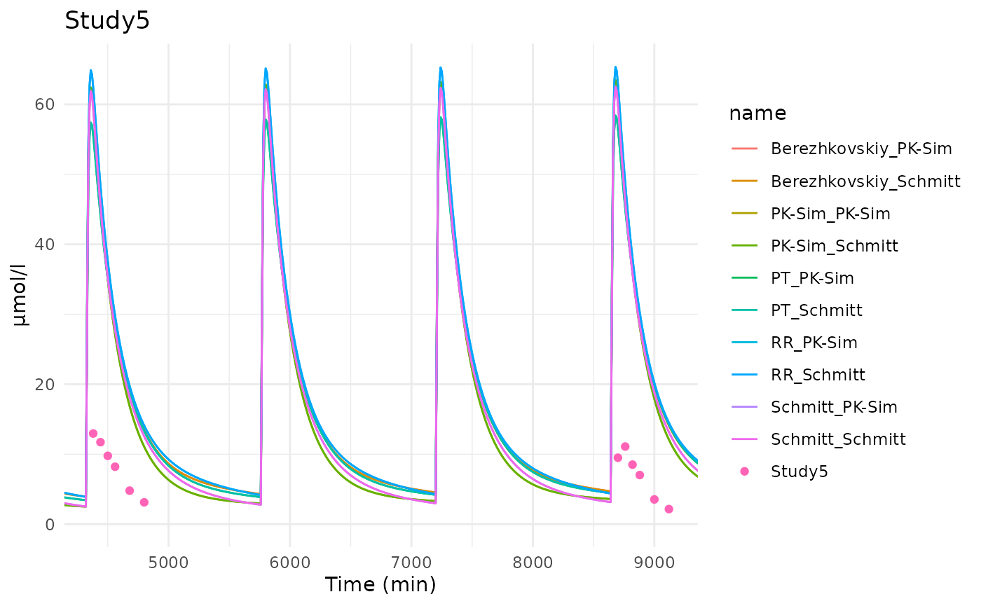
p <- plotPK(
  results = results,
  obsData = dataSets,
  studyID = "Study21",
  outputPath = "Organism|PeripheralVenousBlood|Compound1|Plasma (Peripheral Venous Blood)"
)

print(p)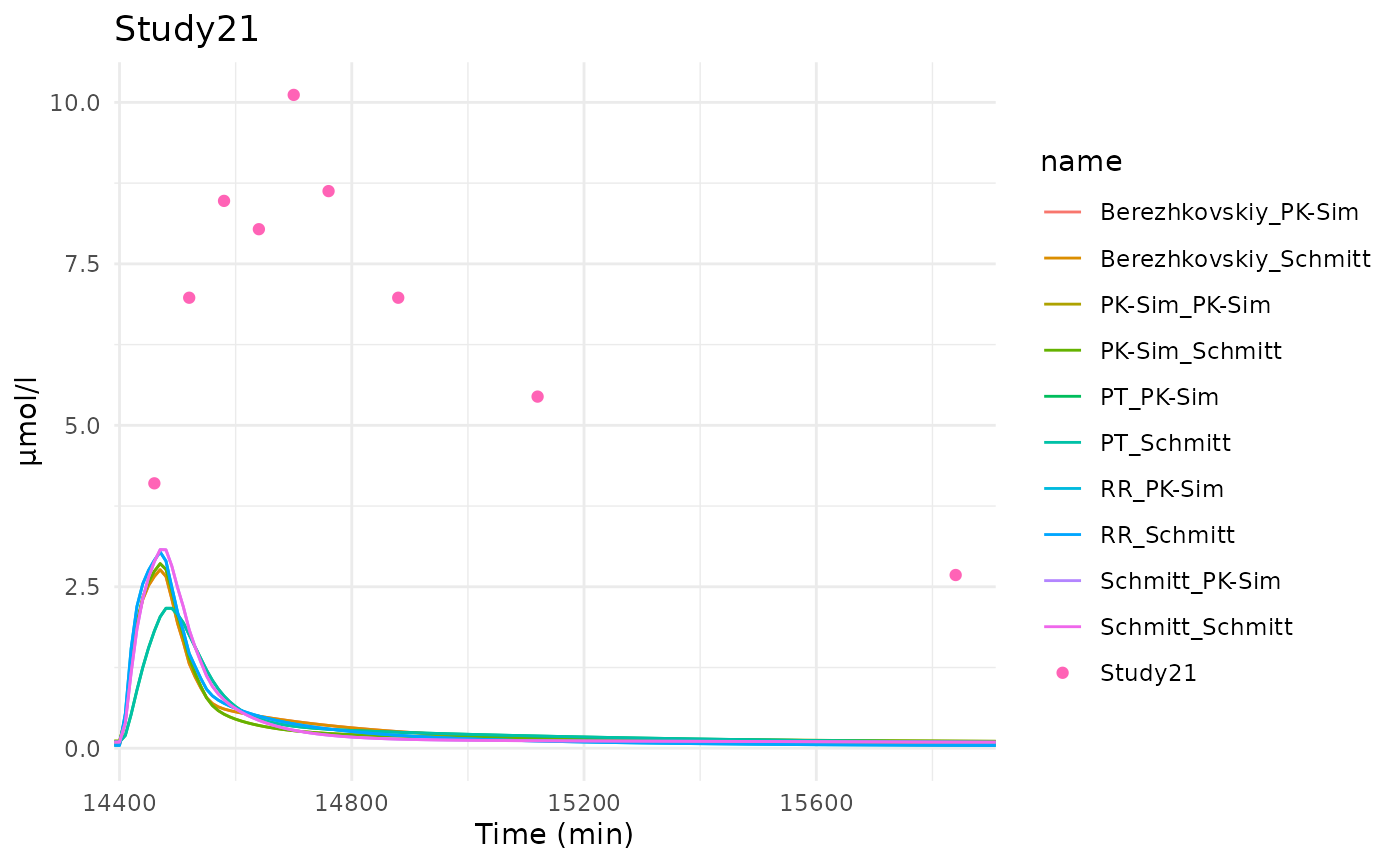
p <- plotPK(
  results = results,
  obsData = dataSets,
  studyID = "Study33",
  outputPath = "Organism|PeripheralVenousBlood|Compound1|Plasma (Peripheral Venous Blood)"
)

print(p)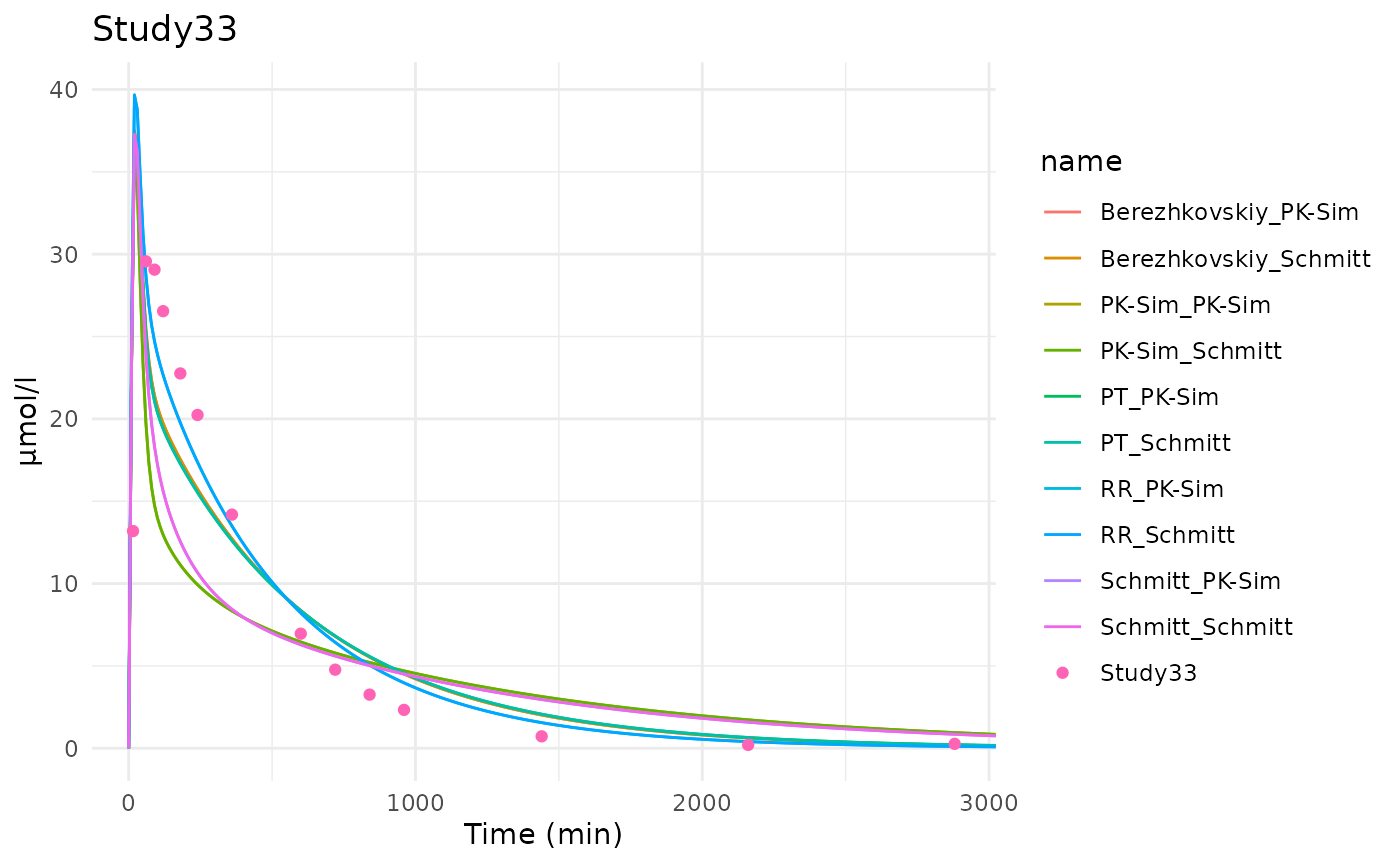
We can easily make a pdf with all studies.
pdf(file.path(outFolder, "Plots.pdf"), width = 6, height = 5)
for (studyID in InputStudies$StudyID) {
  p <- plotPK(
    results = results,
    obsData = dataSets,
    studyID = studyID,
    outputPath = "Organism|PeripheralVenousBlood|Compound1|Plasma (Peripheral Venous Blood)"
  )
  print(p)
}
dev.off()
Let’s look at the overall metrics results across studies and compare the different PC/CP methods. For the anti-TB drug overall the AUC ratio tend to be slightly underpredicted while the Cmax ratio is slightly overpredicted. However the PC/CP methods only have a minor impact on the results probably because the pKa values have not been taken into account.
p <- ggplot(metric_results) +
  geom_boxplot(aes(y = AUCfold, x = method)) +
  scale_y_log10() +
  geom_hline(yintercept = 0.5, linetype = "dashed") +
  geom_hline(yintercept = 2, linetype = "dashed") +
  theme_bw() +
  theme(axis.text.x = element_text(angle = 45, hjust = 1))
p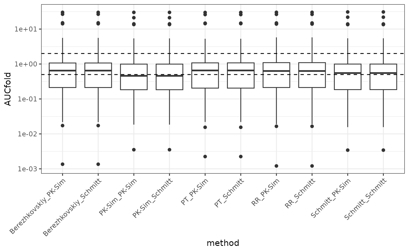
p <- ggplot(metric_results) +
  geom_boxplot(aes(y = cMaxFold, x = method)) +
  scale_y_log10() +
  geom_hline(yintercept = 0.5, linetype = "dashed") +
  geom_hline(yintercept = 2, linetype = "dashed") +
  theme_bw() +
  theme(axis.text.x = element_text(angle = 45, hjust = 1))
p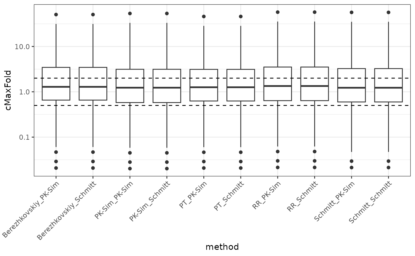
Let’s look at how many studies have an AUC or Cmax within 2 fold of the observed values. With all methods we have around 40% of the studies with an AUC within 2 fold and around 50-60% of the studies with a AUC within 4 fold. Similarly we have 40% of the studies with an Cmax within 2 fold and around 75% of the studies with a Cmax within 4 fold.
tmp <- metric_results %>%
  mutate(
    AUC2fold = AUCfold <= 2 & AUCfold >= 0.5,
    Cmax2fold = cMaxFold <= 2 & cMaxFold >= 0.5,
    AUC4fold = AUCfold <= 4 & AUCfold >= 1/4,
    Cmax4fold = cMaxFold <= 4 & cMaxFold >= 1/4,
  ) %>%
  select(method, AUC2fold, Cmax2fold, AUC4fold, Cmax4fold) %>%
  group_by(method) %>%
  summarize_all(.funs = ~ sum(.x) / n() * 100)
However some compound might have more studies than other, for a fairer comparison we will look after first average per compound. When first averaging per compound we see similar results, mean AUC is within 2 fold for ~42% of the compounds, and within 4-folds for half of them, while cMax is within 2-fold for 1/3 to 42% of the compounds and within 4 fold for around 2/3 to 75 % of the compounds.
tmp <- metric_results %>%
  group_by(Compound, method) %>%
  select(AUCfold, cMaxFold) %>%
  summarise_all(mean, ) %>%
  group_by(method) %>%
  select(-Compound) %>%
  mutate(
    AUC2fold = AUCfold <= 2 & AUCfold >= 0.5,
    Cmax2fold = cMaxFold <= 2 & cMaxFold >= 0.5,
    AUC4fold = AUCfold <= 4 & AUCfold >= 1/4,
    Cmax4fold = cMaxFold <= 4 & cMaxFold >= 1/4,
  ) %>%
  summarize_all(.funs = ~ sum(.x) / n() * 100)
#> Adding missing grouping variables: `Compound`, `method`
If we look at the result for Poulin and Thiel partition coefficient method and PK-Sim cellular permeability method in more details, we see some correlation between AUC ratio and Cmax ratio.
p <- ggplot(metric_results %>% filter(method == "PT_PK-Sim")) +
  geom_point(aes(y = AUCfold, x = cMaxFold, color = Compound), alpha = 0.5, size = 3) +
  scale_y_log10(breaks = c(0.01, 0.05, 0.10, 0.2, 0.5, 1, 2, 5, 10, 20)) +
  scale_x_log10(breaks = c(0.01, 0.05, 0.10, 0.2, 0.5, 1, 2, 5, 10, 20)) +
  geom_hline(yintercept = 0.5, linetype = "dashed") +
  geom_hline(yintercept = 2, linetype = "dashed") +
  geom_vline(xintercept = 0.5, linetype = "dashed") +
  geom_vline(xintercept = 2, linetype = "dashed") +
  theme_bw()

ggplotly(p)
We can also notice that most studies with the same compounds cluster together, indicating that the over/under prediction is compound not due to a particular study design (except one for bedaquiline that has a very long follow up compared to the other study over emphasizing the underprediction of the AUC).
p <- ggplot(metric_results %>% filter(method == "PT_PK-Sim")) +
  geom_boxplot(aes(y = AUCfold, x = Compound, fill = Compound)) +
  scale_y_log10(breaks = c(0.01, 0.05, 0.10, 0.2, 0.5, 1, 2, 5, 10, 20)) +
  geom_hline(yintercept = 2, linetype = "dashed") +
  geom_hline(yintercept = 0.5, linetype = "dashed") +
  theme_bw() +
  theme(axis.text.x = element_text(angle = 45, hjust = 1))
p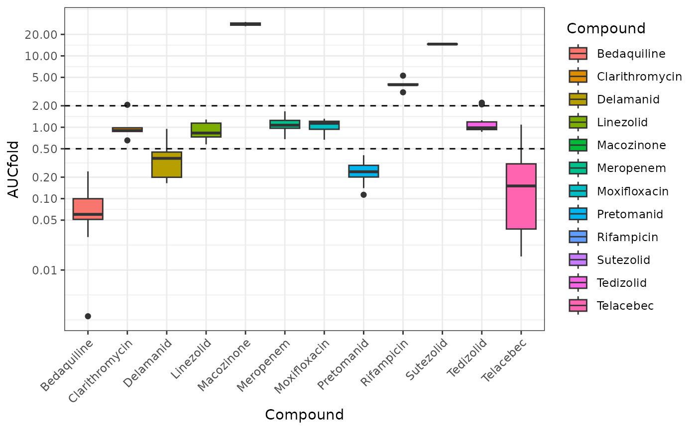
p <- ggplot(metric_results %>% filter(method == "PT_PK-Sim")) +
  geom_boxplot(aes(y = cMaxFold, x = Compound, fill = Compound)) +
  scale_y_log10(breaks = c(0.01, 0.05, 0.10, 0.2, 0.5, 1, 2, 5, 10, 20)) +
  geom_hline(yintercept = 2, linetype = "dashed") +
  geom_hline(yintercept = 0.5, linetype = "dashed") +
  theme_bw() +
  theme(axis.text.x = element_text(angle = 45, hjust = 1))
p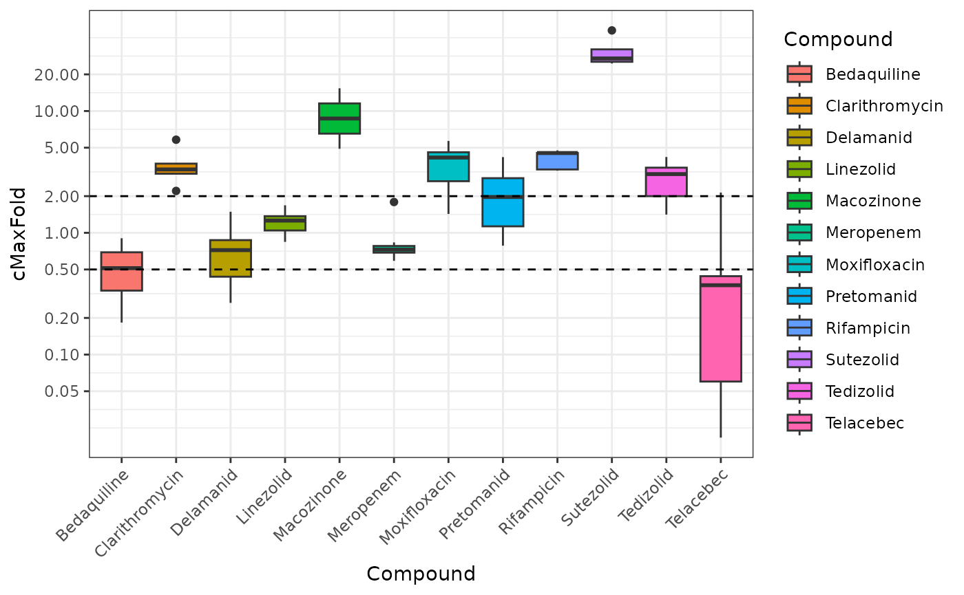
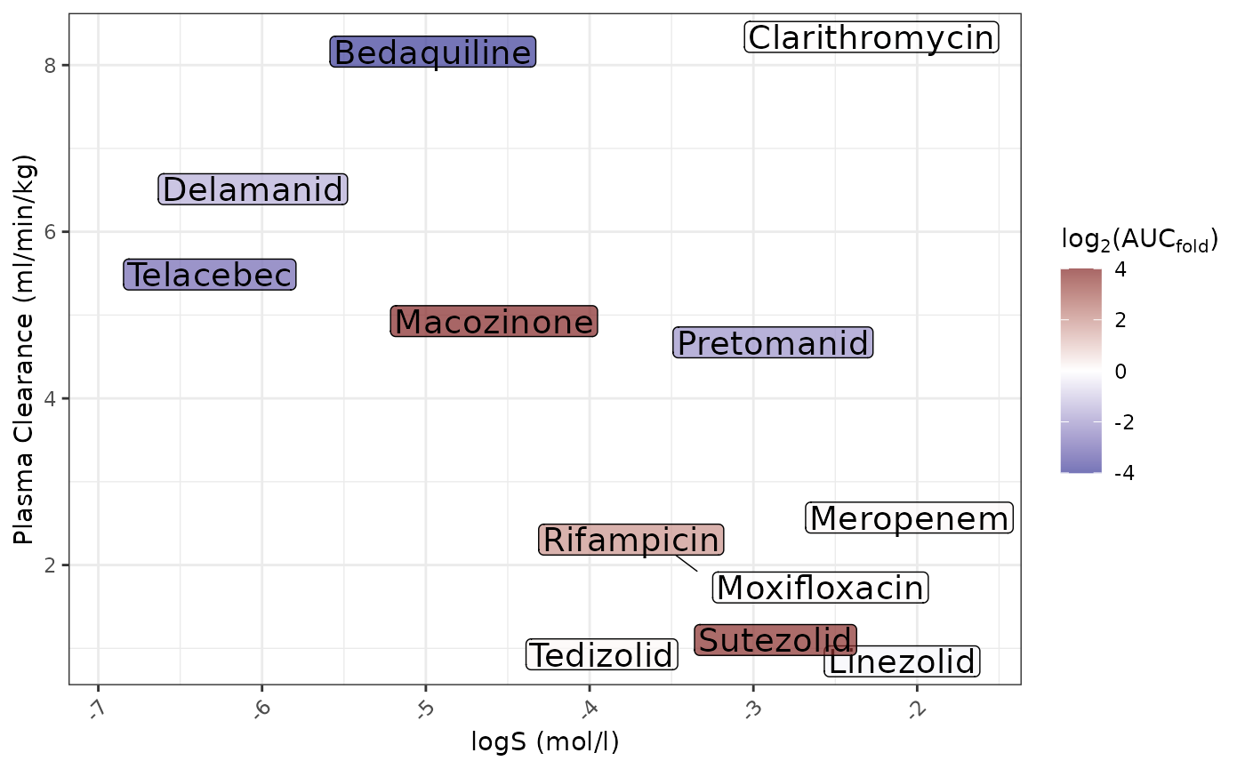
If we look at the inputs to understand what drives the over/under prediction we can see that compounds with high lipophilicity or low fraction unbound, as well as low solubility are less well predicted.
# add compound properties to metric results
metric_results$Lipo <- InputCompounds$`logD - ADMETLab (mol/l)`[match(metric_results$Compound, InputCompounds$Compound)]
metric_results$Solubility <- InputCompounds$`logS - ADMETLab (mol/l)`[match(metric_results$Compound, InputCompounds$Compound)]
metric_results$PInt <- InputCompounds$`logMDCK - ADMETLab (cm/s)`[match(metric_results$Compound, InputCompounds$Compound)]
metric_results$MW <- InputCompounds$`MW (g/mol)`[match(metric_results$Compound, InputCompounds$Compound)]
metric_results$Fu <- InputCompounds$`Fu - ADMETLab`[match(metric_results$Compound, InputCompounds$Compound)]
metric_results$Cl <- InputCompounds$`cl-plasma - ADMETLab (ml/min/kg)`[match(metric_results$Compound, InputCompounds$Compound)]
p <- metric_results %>%
  filter(method == "PT_PK-Sim") %>%
  summarise(log2AUCfold_avg = mean(log2(AUCfold)), .by = c(Compound, Lipo, Cl, Fu, Solubility, PInt, MW)) %>%
  ggplot +
  scale_fill_gradient2(
    low = alpha(muted("blue"), 0.7),
    mid = alpha("white",0.7),
    high = alpha(muted("red"), 0.7),
    midpoint = 0,
    limits = c(-4, 4),
    oob = scales::squish
  ) +
  geom_label_repel(
    mapping = aes(y = Fu, x = Lipo, label = Compound, fill = log2AUCfold_avg),
    label.size = NA,
    size = 5,
    segment.size = 0.25,
    label.padding = 0.1
  ) +
  theme_bw() +
  theme(axis.text.x = element_text(angle = 45, hjust = 1)) +
  labs(y = "Fraction unbound (%)", x = "LogD", fill = bquote(log[2]*"("*AUC[fold]*")"))

p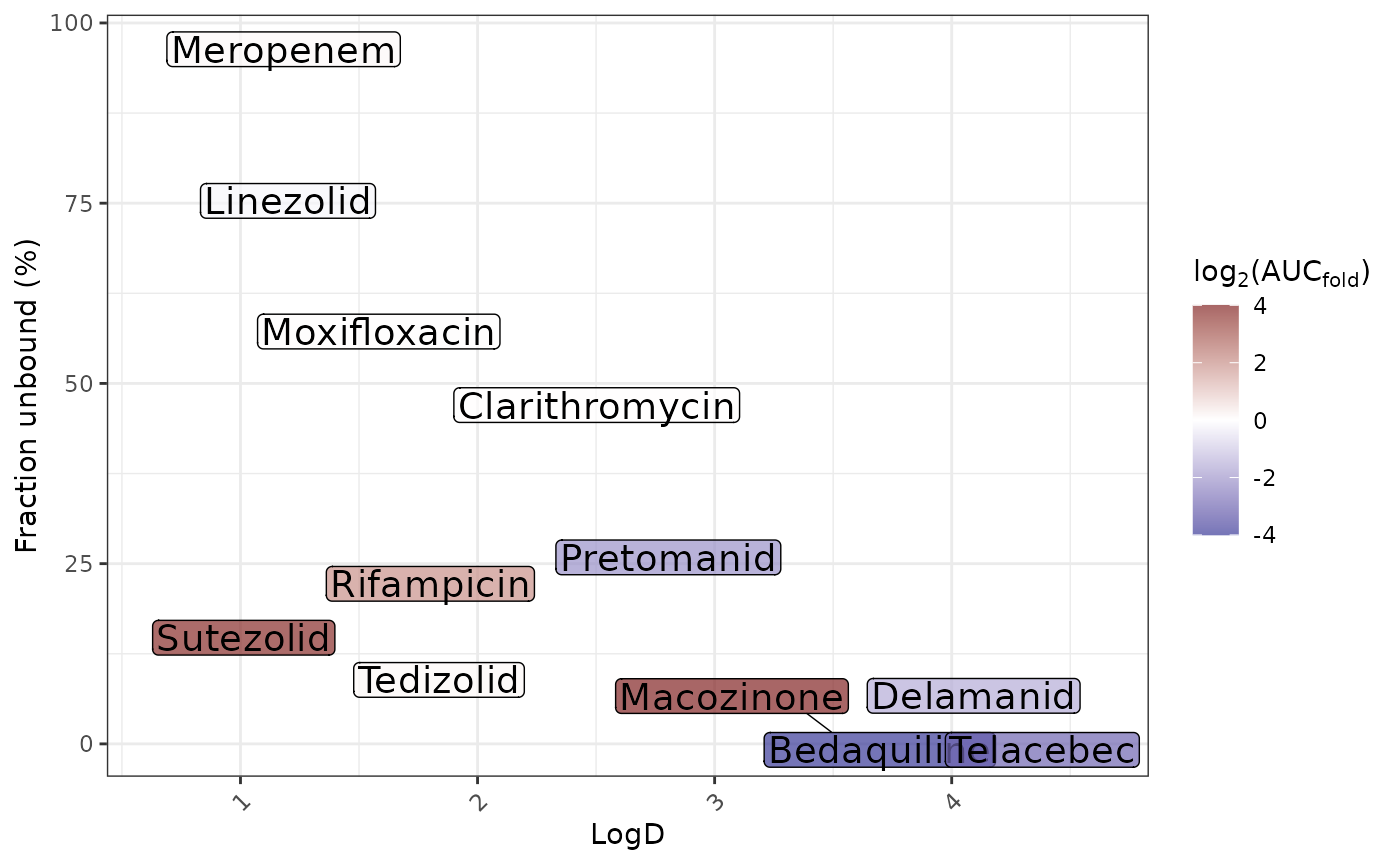
p <- metric_results %>%
  filter(method == "PT_PK-Sim") %>%
  summarise(log2AUCfold_avg = mean(log2(AUCfold)), .by = c(Compound, Lipo, Cl, Fu, Solubility, PInt, MW)) %>%
  ggplot() +
  scale_fill_gradient2(
    low = alpha(muted("blue"), 0.7),
    mid = alpha("white",0.7),
    high = alpha(muted("red"), 0.7),
    midpoint = 0,
    limits = c(-4,4),
    oob = scales::squish
  ) +
  geom_label_repel(
    mapping = aes(y = Cl, x = Solubility, label = Compound, fill = log2AUCfold_avg),
    label.size = NA,
    size = 5,
    segment.size = 0.25,
    label.padding = 0.1
  ) +
  theme_bw() +
  theme(axis.text.x = element_text(angle = 45, hjust = 1)) +
  labs(x = "logS (mol/l)", y = "Plasma Clearance (ml/min/kg)", fill = bquote(log[2]*"("*AUC[fold]*")"))
p