Example with chembl dataset
Example-with-chembl-dataset.RmdLoad needed libraries
For this example we will load a few libraries
library(ESQhtpbpk) # package for HTPBPK
library(readxl) # package to read xlsx files that contains input data
library(dplyr) # package for easy manipulation of data
library(tidyr) # package for easy manipulation of data
library(stringr) # package for string manipulation
# packages for plotting
library(ggplot2)
library(plotly)
# packages for parallel computing
library(doParallel)
Load input files
A dataset of Cmax and AUC values, extracted and curated from CHEMBL, is available in the package as an example dataset.
# Reading curated chembl dataset with AUC and Cmax values
path <- system.file(
  "extdata",
  "Chembl_preprocessed_curated.xlsx",
  package = "ESQhtpbpk"
)
The first sheet of the excel file lists the studies and the observed data available for each study.
# Reading curated chembl dataset with AUC and Cmax values
InputStudies <- read_excel(path, sheet = 1)
The second sheet of the excel file lists the protocol information to be simulated. A protocol can span multiple lines for the same study, for example, in the case of multiple administrations with a loading dose.
InputProtocol <- read_excel(path, sheet = 2)The third sheet of the excel file lists all the compound properties. Based on this paper and specifically Table 1, we extracted compound properties from ADMETlab QSAR as input to the HT-PBPK model.
InputCompounds <- read_excel(path, sheet = 3) # QSARs obtained from ADMETlab 3.0Summary of compound properties included in the dataset
This dataset was extracted from Chembl and further curated to include only studies with a single compound administered to healthy adults, where AUC or Cmax data were available, and the protocol was identified from the original publication.
With the careful curation, the dataset contains 48 compounds.
Here is a summary of the properties for included compounds:
InputCompounds %>%
  pivot_longer(
    cols = c(MW, logP, logD, logS, Fu, PPB, MDCK, caco2, PAMPA,
             `cl-plasma`, pka_acidic, pka_basic),
    names_to = "Property",
    values_to = "Value"
  ) %>%
  ggplot() +
    geom_histogram(aes(x = Value)) +
    facet_wrap(~ Property, scales = "free")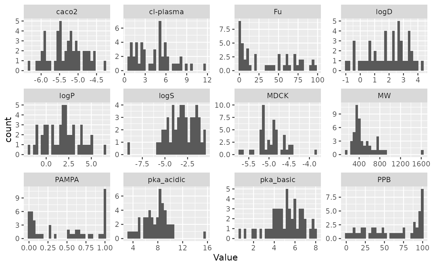
Testing multiple scenarios
The platform allows easy testing of multiple scenarios by adjusting inputs as needed based on the selected conditions. An example Excel file with different scenarios is available in the package. For example, solubility can be set to an arbitrarily high value or to the value from QSAR. Lipophilicity can be set to logP or logD, etc.
scenarios <- read.csv(
  file = system.file(
    "extdata",
    "Chembl_Test_Pipeline",
    "scenarios.csv",
    package = "ESQhtpbpk"
  ),
  stringsAsFactors = FALSE
)
The various scenarios can be easily implemented when setting up the compound by using if or switch conditions when setting the inputs (see below).
Running the pipeline
First, we set the output folder where the results will be saved.
outputFolder <- "Chembl_Test_Pipeline"
dir.create(outputFolder, showWarnings = FALSE)
To create studies, it depends on how the inputs are formatted. It can be very useful to create custom functions tailored to these inputs.
Compound creation for various scenarios
First, let’s create a custom function that will create a compound object based on our inputs and the scenario tested. It will then be easy to wrap this to create all the studies needed for all the scenarios we want.
createCompound <- function(chembl_id, scenario) {
  compoundIdx <- which(InputCompounds$molecule_chembl_id == chembl_id)

  # Set new compound with compound name corresponding to chembl_id
  comp <- Compound$new(ID = chembl_id)

  # if halogens are considered set halogenes numbers
  if (scenario$Halogen == 1) {
    # Set halogen numbers (up to 10 allowed in PK-Sim)
    comp$setPropertyValue(
      "Chlorine count",
      value = min(10, str_count(InputCompounds$smiles[compoundIdx], "Cl"))
    )
    comp$setPropertyValue(
      "Bromine count",
      value = min(10, str_count(InputCompounds$smiles[compoundIdx], "Br"))
    )
    comp$setPropertyValue(
      "Fluorine count",
      value = min(10, str_count(InputCompounds$smiles[compoundIdx], "F"))
    )
    comp$setPropertyValue(
      "Iodine count",
      value = min(10, str_count(InputCompounds$smiles[compoundIdx], "I"))
    )
  }

  # set molecular weight
  comp$setPropertyValue(
    "Molecular weight",
    value = InputCompounds$MW[compoundIdx],
    unit = "g/mol"
  )

  # Set solubility depending on scenario
  comp$setPropertyValue(
    "Solubility",
    value = switch(
      as.character(scenario$Solubility),
      # set solubility from QSAR
      # ADMETlab logS QSAR is given as log10 of mol/l, convert to g/l for PK-Sim
      logS = 10 ^ InputCompounds$logS[compoundIdx] * InputCompounds$MW[compoundIdx],
      # set arbitrary high solubility
      High = 1000
    ),
    unit = "g/l"
  )

  # Set lipophilicity based on scenario
  comp$setPropertyValue(
    "Lipophilicity",
    value = switch(
      as.character(scenario$Lipophilicity),
      # set  lipophilicity to logP
      logP = InputCompounds$logP[compoundIdx],
      # set  lipophilicity to logD
      logD = InputCompounds$logD[compoundIdx],
      # use logMA as lipophilicity input
      logMA1 = 1.294 + 0.304 * InputCompounds$logP[compoundIdx],
      # use logMA as lipophilicity input
      logMA_Pearce = 0.0166 * 37 + 0.882 * InputCompounds$logP[compoundIdx]
    ),
    unit = "Log Units"
  )

  # Set Fu based on scenario
  comp$setPropertyValue(
    "Fraction unbound",
    value = switch(
      as.character(scenario$Fu),
      # use Fu QSAR
      Fu = InputCompounds$Fu[compoundIdx],
      # use PPB QSAR
      PPB = 100 - InputCompounds$PPB[compoundIdx]
    ),
    unit = "%"
  )

  # Set intestinal permeability based on scenario
  # intestinal permeability is not predefined it needs to be added with addProperty
  if (scenario$Pint != "PK-Sim") {
    comp$addProperty(
      name = "PInt",
      parName = "Specific intestinal permeability (transcellular)",
      dimension = "Velocity",
      value = switch(
        as.character(scenario$Pint),
        # set Pint to MDCK QSAR value
        MDCK = 10^InputCompounds$MDCK[compoundIdx], # MDCK is in log cm/s,
        # set Pint to Caco2 QSAR value
        Caco2 = 10^InputCompounds$caco2[compoundIdx], # Caco2 is in log cm/s,
        # set Pint to PAMPA QSAR value
        PAMPA = InputCompounds$PAMPA[compoundIdx] * 1e-6 # PAMPA is in 10E-6 cm/s,
      ),
      unit = "cm/s"
    )
  }

  # Set organ permeability to arbitrarily high value if scenario requires it
  if (scenario$Perm ==  "High") {
    comp$addProperty(
      name = "Perm",
      parName = "Permeability",
      dimension = "Velocity",
      value = 10,
      unit = "cm/s"
    )
  }

  # Add total clearance (as hepatic clearance) also add matching fu and lipophilicity
  comp$addProcessProperty(
    processType = "Liver Plasma Clearance",
    propertyName = "Plasma clearance",
    parName = "Plasma clearance",
    dimension = "Flow per weight",
    value = InputCompounds$`cl-plasma`[compoundIdx],
    unit = "ml/min/kg"
  )
  comp$addProcessProperty(
    processType = "Liver Plasma Clearance",
    propertyName = "Lipophilicity",
    parName = "Lipophilicity (experiment)",
    dimension = "Log Units",
    value = suppressMessages(comp$getProperty("Lipophilicity")$value),
    unit = suppressMessages(comp$getProperty("Lipophilicity")$unit)
  )
  comp$addProcessProperty(
    processType = "Liver Plasma Clearance",
    propertyName = "Fraction unbound",
    parName = "Fraction unbound (experiment)",
    dimension = "Fraction",
    value = suppressMessages(comp$getProperty("Fraction unbound")$value),
    unit = suppressMessages(comp$getProperty("Fraction unbound")$unit)
  )

  # Consider pka depending on scenario (restrict to 0-14 range)
  if (scenario$PkA == 1) {
    comp$setPropertyValue(
      name = "pKa value 0",
      value = min(max(c(0,InputCompounds$pka_acidic[compoundIdx])), 14)
    )
    comp$setPropertyValue("Compound type 0", "Acidic")

    comp$setPropertyValue(
      name = "pKa value 1",
      value = min(max(c(0,InputCompounds$pka_basic[compoundIdx])), 14)
    )
    comp$setPropertyValue("Compound type 1", "Basic")
  }

  # Include default GFR fraction of 1 based on scenario
  if (scenario$GFR == 1) {
    comp$addProcessProperty(
      processType = "GFR",
      propertyName = "GFR",
      parName = "GFR fraction",
      dimension = "Dimensionless",
      value = 1
    )
  }

  # Set liver enzyme concentration to 1 umol/l in
  # intracellular space if enzyme correction tested
  if (scenario$Enzyme_correction == 1) {
    comp$addProcessProperty(
      processType = "Liver Plasma Clearance",
      propertyName = "Enzyme correction",
      parName = "Enzyme concentration",
      dimension = "Concentration (molar)",
      value = 1/0.667, # 1/0.667 is the correction factor for the enzyme activity
      unit = "umol/l"
    )
  }

  return(comp)
}
Protocol creation
We can also create a custom function to define our administration protocols based on how our protocol information is set up.
createProtocol <- function(protocol_id, scenario) {
  # extract lines corresponding to the wanted protocol
  protocolTable <- InputProtocol[InputProtocol$ProtocolID == protocol_id,]

  # create advanced protocol (1 protocol can be defined by multiple lines
  # in the excel with different admin, for example with loading dose)
  prot <- AdvancedProtocol$new()

  # skip if some dose is not available (look depending on scenario selected)
  doseVal <- switch(
    as.character(scenario$Dose),
    Flat = protocolTable$`Dose`,
    BW = protocolTable$`Dose Norm`
  )
  doseUnit <- switch(
    as.character(scenario$Dose),
    Flat = protocolTable$`Dose Unit`,
    BW = protocolTable$`Dose Norm Unit`
  )

  if (any(is.na(doseVal) | is.na(doseUnit))) {
    return(NULL)
  }

  # Add schema for each line of the protocol info
  for (i in seq_len(nrow(protocolTable))) {
    # default is 1 dose, with 0 time between repetitions if not specified
    prot$addSchema(
      schemaName = paste0("Schema_", i),
      startTime = protocolTable$Time[i],
      timeBetweenRepetitions = protocolTable$Time_between_rep[i] %>% ifelse(is.na(.), 0, .),
      numberOfRepetitions = protocolTable$Nrep[i] %>% ifelse(is.na(.), 1, .),
      timeUnit = protocolTable$TimeUnit[i]
    )

    # select dose type based on scenario (dose as given, or always converted to per kg)
    admin <- SimpleProtocol$new(
      # match route from excel to allowed route in package
      route = c("ORAL" = "Oral", "IV INFUSION" = "IV Infusion")[protocolTable$Route[i]],
      dose = doseVal[i],
      doseUnit = doseUnit[i],
      infusionTime = (protocolTable$Infusion_duration[i] %>% if (is.na(.)) NULL else .),
      infusionTimeUnit = (protocolTable$Infusion_duration_unit[i] %>% if (is.na(.)) NULL else .)
    )

    # for oral admin assume dissolved formulation
    if (protocolTable$Route[i] == "Oral") {
      formulation <- createDissolvedFormulation(name = "Dissolved")
      admin$setFormulation(formulation = formulation)
    }

    # add schema to protocol
    prot$addProtocolToSchema(admin, schemaName = paste0("Schema_", i))
  }

  return(prot)
}
Studies creation
Then, we can easily use these function to create the list of studies for each scenario we want to test.
createStudies <- function(scenario) {

  # initialise to an empty list of studies
  Studies <- list()

  # we loop over all compounds (for faster execution,
  # as that way the compound will need to be created only once)
  # we could also loop over the studies but then for each study
  # the compound would need to be created again

  for (compoundIdx in seq_len(nrow(InputCompounds))) {
    # create compound with inputs matching wanted scenario
    compChemblId <- InputCompounds$molecule_chembl_id[compoundIdx]

    comp <- createCompound(
      chembl_id = compChemblId,
      scenario = scenario
    )

    # create studies using the compound (as in our case studies only use a single compound)
    # our input data as 1 ine per observation hence the use of unique function
    studyIdsForComp <- unique(
      InputStudies$StudyID[which(InputStudies$molecule_chembl_id == compChemblId)]
    )
    for (studyId in studyIdsForComp) {
      print(studyId)
      studyIdx <- which(InputStudies$StudyID == studyId)

      # create protocol for the study
      prot <- createProtocol(
        protocol_id = unique(InputStudies$ProtocolID[studyIdx]),
        scenario = scenario
      )

      if (is.null(prot)) {
        # skip if no protocol available (i.e. missing dose information
        # for example for BW norm dose if BW was not available)
        next()
      }

      # set protocol to the compound
      comp$setProtocol(prot)

      # set wanted PC and CP method
      comp$PartitionCoefficientMethod <- "PK-Sim"
      comp$CellularPermeabilityMethod <- "PK-Sim"

      # create study with the compound and protocol for human individual
      study <- Study$new(
        ID = paste(studyId, comp$PartitionCoefficientMethod, comp$CellularPermeabilityMethod, sep = "_"),
        compounds = list(comp),
        individual = "Human"
      )

      # add to the list of studies
      Studies <- c(Studies, study)
    }
  }
  # add studies ID as names to the list of studies
  names(Studies) <- sapply(Studies, function(x) x$ID)

  return(Studies)
}
Simulating the studies
Once we have created the studies, we can run the simulation. Let’ s run the studies for the first scenario.
studies <- createStudies(scenario = scenarios[1, ])

# Create folder to save the the pkml and results if wanted and run the simulations
outputFolderScenario <- file.path(outputFolder, "Chembl_Scenario_1")
dir.create(outputFolderScenario, showWarnings = FALSE)

# run Predictions for compound plasma in PVB
results <- runPredictions(
  studies,
  outputFolder = outputFolderScenario,
  numberOfCores = 5,
  outputSelections = c("Organism|PeripheralVenousBlood|**|Plasma (Peripheral Venous Blood)"),
  simulationResolution = c(0, max(InputStudies$`t_end [h]`) * 60, 0.1),
  saveResults = FALSE,
  saveSimulation = FALSE,
  queueSize = 200
)
Calculating prediction metrics
The output metrics must be customized to those required for the specific analysis. Here, we calculate various AUC and Cmax metrics based on our HT-PBPK predictions using the PKNCA package, matched to the observed dataset.
The metrics depend on the observed data we have, so this part will also be adjusted to one’s specific needs.
Since we need to calculate the metrics for multiple studies and scenarios, it can be helpful to create a function that performs the calculations.
calculateMetrics <- function(study, simData, obsData) {
  # if needed convert time unit to match obs data time unit in our case all time are in hours
  simData$data$Time <- ospsuite::toUnit(
    quantityOrDimension = simData$metaData$Time$dimension,
    values = simData$data$Time,
    sourceUnit = simData$metaData$Time$unit,
    targetUnit = "h"
  )
  simData$metaData$Time$unit <- "h"

  # add compound molecular weight to the metadata to ensure conversion of umol/l to g/l if needed
  simData$metaData$MW <- list(
    value = suppressMessages(study$Compounds[[1]]$getProperty("Molecular weight")$value),
    unit = suppressMessages(study$Compounds[[1]]$getProperty("Molecular weight")$unit)
  )

  # Initialise result vector
  SimMetric <- c()

  # calculate metrics for each observed data (a single study can have multiple observed data)
  for (i in seq_len(nrow(obsData))) {
    if (obsData[i,]$Metric %in% c("AUC", "Cmax")) {
      # Filter time required to calculate the AUC from the correct time interval (e.g. restrict
      # to 0:24h for AUC024, restrict to 0 to end of sim for AUC0Inf, or to the last dose interval
      # for Cmax of last dose, ...)
      simDataToUse <- simData$data %>%
        dplyr::filter(
          Time <= min(obsData[i,]$`t_end [h]`, as.numeric(obsData[i,]$`Metric_t2 [h]`)),
          Time >= obsData[i,]$`Metric_t1 [h]`
        )
    } else {
      # In our case the only other metric is Concentration at a specific timepoint
      simDataToUse <- simData$data
    }

    if (obsData[i,]$Metric == "AUC") {
      # calculate AUC with PKNCA (suppress no dose given warning as not required for auc)
      resPred <- suppressWarnings(
        PKNCA::pk.nca(
          PKNCA::PKNCAdata(
            data.conc = PKNCA::PKNCAconc(
              simDataToUse, `Organism|PeripheralVenousBlood|Compound1|Plasma (Peripheral Venous Blood)` ~ Time|IndividualId
            ),
            intervals = data.frame(
              start = obsData[i,]$`Metric_t1 [h]`,
              end = as.numeric(obsData[i,]$`Metric_t2 [h]`),
              auclast = TRUE,
              aucinf.pred = TRUE,
              aucinf.obs = FALSE,
              half.life = FALSE
            )
          )
        )
      )

      # get PKNCA results
      if (is.finite(as.numeric(obsData[i,]$`Metric_t2 [h]`))) {
        # for AUC t1 to finite time
        resPred <- resPred$result %>% filter(PPTESTCD == "auclast") %>% pull(PPORRES)
      } else {
        if (!is.na(resPred$result %>% filter(PPTESTCD == "aucinf.pred") %>% pull(PPORRES))) {
          # for AUC t1 to Inf
          resPred <- resPred$result %>% filter(PPTESTCD == "aucinf.pred") %>% pull(PPORRES)
        } else {
          # if na it means to the simdata was still increase at the end of the observed data time-frame,
          # try calculating AUC0Inf using all simulation time frame
          simDataToUse <- simData$data %>%
            dplyr::filter(
              Time <= as.numeric(obsData[i,]$`Metric_t2 [h]`),
              Time >= obsData[i,]$`Metric_t1 [h]`
            )
          # calculate AUC with PKNCA (up to end of simulation instead of end of observed data)
          resPred <- suppressWarnings(
            PKNCA::pk.nca(
              PKNCA::PKNCAdata(
                data.conc = PKNCA::PKNCAconc(
                  simDataToUse, `Organism|PeripheralVenousBlood|Compound1|Plasma (Peripheral Venous Blood)` ~ Time|IndividualId
                ),
                intervals = data.frame(
                  start = obsData[i,]$`Metric_t1 [h]`,
                  end = as.numeric(obsData[i,]$`Metric_t2 [h]`),
                  auclast = TRUE,
                  aucinf.pred = TRUE,
                  aucinf.obs = FALSE,
                  half.life = FALSE
                )
              )
            )
          )

          if (!is.na(resPred$result %>% filter(PPTESTCD == "aucinf.pred") %>% pull(PPORRES))) {
            # for AUC t1 to Inf
            resPred <- resPred$result %>% filter(PPTESTCD == "aucinf.pred") %>% pull(PPORRES)
          } else {
            # if still na, i.e still increasing at end of simulation timeframe set to AUClast
            resPred <- resPred$result %>% filter(PPTESTCD == "auclast") %>% pull(PPORRES)
          }
        }
      }

      # convert to the observed unit
      resPred <- ospsuite::toUnit(
        quantityOrDimension = ospsuite::getDimensionForUnit(obsData[i,]$OspUnits),
        values = resPred,
        # add "*" time unit to the simulated concentration unit to unit to make compatible AUC units
        sourceUnit = gsub(
          pattern = "/",
          replacement = paste0("*", simData$metaData$Time$unit, "/"),
          x = simData$metaData$`Organism|PeripheralVenousBlood|Compound1|Plasma (Peripheral Venous Blood)`$unit,
        ),
        targetUnit = obsData[i,]$OspUnits,
        molWeight = simData$metaData$MW$value,
        molWeightUnit = simData$metaData$MW$unit
      )

    } else if (obsData[i,]$Metric %in% c("Cmax", "C")) {
      # convert to same unit as observed data
      resPred <- ospsuite::toUnit(
        quantityOrDimension = simData$metaData$`Organism|PeripheralVenousBlood|Compound1|Plasma (Peripheral Venous Blood)`$dimension,
        values = simDataToUse$`Organism|PeripheralVenousBlood|Compound1|Plasma (Peripheral Venous Blood)`,
        sourceUnit = simData$metaData$`Organism|PeripheralVenousBlood|Compound1|Plasma (Peripheral Venous Blood)`$unit,
        targetUnit = obsData[i,]$OspUnits,
        molWeight = simData$metaData$MW$value,
        molWeightUnit = simData$metaData$MW$unit
      )

      if (obsData[i,]$Metric  == "Cmax") {
        resPred <- max(resPred)
      } else {
        # interpolate to get value at time
        resPred <- approx(
          x =  simData$data$Time,
          y =  resPred,
          xout = obsData[i,]$`Metric_t1 [h]`,
          rule = 2
        )
        resPred <- resPred$y
      }
    }
    SimMetric <- c(SimMetric, resPred)
  }

  return(cbind(obsData, SimMetric  = SimMetric))
}
Now that we created the function calculate the metrics on our simulated data, we can run it for each study result in parallel and save as a csv file.
# create and register parallel backend for calculating the metric needed
# to compare to the observed data faster
cl <- makePSOCKcluster(5)
registerDoParallel(cl)

# get predicted values from the HT-PBPK run first as it cannot be access from parallel workers
simData <- lapply(results, function(studyResult) {
  ospsuite::getOutputValues(studyResult, individualIds = results$allIndividualIds)
})

# Calculate observed metrics on the predicted curves in parallel
metric_results <- foreach::foreach(
  studyID = unique(InputStudies$StudyID),
  .combine = rbind,
  .packages = c("dplyr", "PKNCA", "ospsuite"),
  .export = c("InputStudies", "calculateMetrics", "simData", "studies"),
  .errorhandling = "pass",
  .verbose = T
) %dopar% {
  simID <- paste(studyID, "PK-Sim Standard", "PK-Sim Standard", sep = "_")

  calculateMetrics(
    study = studies[[simID]],
    simData = simData[[simID]],
    obsData = InputStudies %>% filter(StudyID == studyID)
  )
}

write.csv(
  metric_results,
  file = file.path(outputFolder, paste0("metrics_scenario_1.csv")),
  row.names = FALSE
)

# stop cluster once done
stopCluster(cl)
Testing multiple scenarios
As demonstrated, it is straightforward to run the pipeline for multiple scenarios to test various QSARs or hypotheses.
# create and register parallel backend for calculating the metric needed
# to compare to the observed data faster
cl <- makePSOCKcluster(5)
registerDoParallel(cl)

# Create studies for each compound and each scenario we want (here we are testing default scenario
# and with increase organ permeability)

for (scenario_row in seq_len(nrow(scenarios))) {
  scenarioNb <- scenarios$Scenario[scenario_row]

  # create studies for the scenario
  studies <- createStudies(scenario = scenarios[scenario_row, ])

  # Create folder to save the the pkml and results if wanted and run the simulations
  outputFolderScenario <- file.path(outputFolder, paste0("Chembl_Scenario_", scenarioNb))
  dir.create(outputFolderScenario, showWarnings = FALSE)

  # run Predictions for compound plasma in PVB
  results <- runPredictions(
    studies,
    outputFolder = outputFolderScenario,
    numberOfCores = 5,
    outputSelections = c("Organism|PeripheralVenousBlood|**|Plasma (Peripheral Venous Blood)"),
    simulationResolution = c(0, max(InputStudies$`t_end [h]`) * 60, 0.1),
    saveResults = FALSE,
    saveSimulation = FALSE,
    queueSize = 200
  )

  # get predicted values from the HT-PBPK run first as it cannot be access from parallel workers
  simData <- lapply(results, function(studyResult) {
    ospsuite::getOutputValues(studyResult, individualIds = results$allIndividualIds)
  })

  # Calculate observed metrics on the predicted curves in parallel
  metric_results <- foreach::foreach(
    studyID = unique(InputStudies$StudyID),
    .combine = rbind,
    .packages = c("dplyr", "PKNCA", "ospsuite"),
    .export = c("InputStudies", "calculateMetrics", "simData", "studies"),
    .errorhandling = "pass",
    .verbose = T
  ) %dopar% {
    simID <- paste(studyID, "PK-Sim Standard", "PK-Sim Standard", sep = "_")

    calculateMetrics(
      study = studies[[simID]],
      simData = simData[[simID]],
      obsData = InputStudies %>% filter(StudyID == studyID)
    )
  }

  write.csv(
    metric_results,
    file = file.path(outputFolder, paste0("metrics_scenario", scenarioNb, ".csv")),
    row.names = FALSE
  )
}

# stop cluster once done
stopCluster(cl)
Looking at the results
Scenario 1
AUC0Inf
The results have already been calculated and are available in the package. You can load them using the following code for the default Scenario 1:
path <- system.file("extdata", "Chembl_Test_Pipeline", "metrics_scenario1.csv", package = "ESQhtpbpk")
metric_results_1 <- read.csv(path, stringsAsFactors = FALSE, check.names = FALSE)
The predictions can be checked against the observed data.
The AUC0Inf for all compounds is centered slightly above 1, meaning that, with the default HT-PBPK and ADMETlab QSAR, it tends to slightly overestimate the AUC compared to the observed value:
metric_results_1 %>%
  filter(Metric == "AUC", `Metric_t1 [h]` == 0, `Metric_t2 [h]` == Inf) %>%
  group_by(molecule_pref_name) %>%
  summarise(
    AUC0InfAvg = mean(Value, na.rm = TRUE),
    AUC0InfPredAvg = mean(SimMetric, na.rm = TRUE),
    AUC0InfRatio = mean(SimMetric / Value, na.rm = TRUE)
  ) %>%
  ggplot() +
    geom_boxplot(aes(y = AUC0InfRatio)) +
    scale_y_log10() +
    theme_bw() +
    theme(aspect.ratio = 5)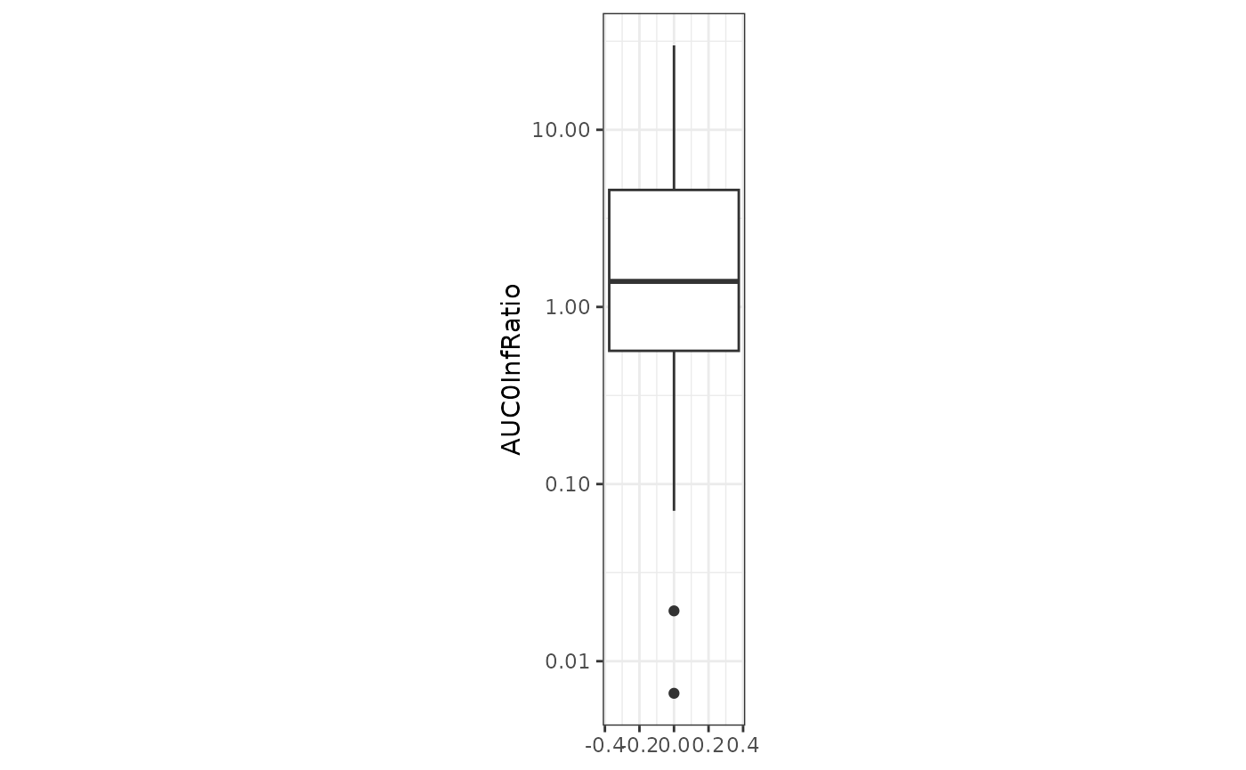
There are 31.1 % of compounds with a predicted AUC0Inf within 2-fold of the observed value, 57.8% within 4-fold and 75.6 % within 10-fold.
We can also look at the AUC0Inf fold ratio for the different percentiles:
tmp <- metric_results_1 %>%
  filter(Metric == "AUC", `Metric_t1 [h]` == 0, `Metric_t2 [h]` == Inf) %>%
  group_by(molecule_pref_name) %>%
  summarise(
    AUC0InfAvg = mean(Value, na.rm = TRUE),
    AUC0InfPredAvg = mean(SimMetric, na.rm = TRUE),
    AUC0InfRatio = mean(SimMetric / Value, na.rm = TRUE)
  ) %>%
  summarise(
    AUC0InfRatio5th = 2^quantile(abs(log2(AUC0InfRatio)), c(0.05)),
    AUC0InfRatio25th = 2^quantile(abs(log2(AUC0InfRatio)), c(0.25)),
    AUC0InfRatio50th = 2^quantile(abs(log2(AUC0InfRatio)), c(0.50)),
    AUC0InfRatio75th = 2^quantile(abs(log2(AUC0InfRatio)), c(0.75)),
    AUC0InfRatio95th = 2^quantile(abs(log2(AUC0InfRatio)), c(0.95))
  )
So We have 50% of the compound for which the AUC0Inf fold ratio is within 3.2 folds.
If we look more in detail at the AUC0Inf (one dot is one studies and one compound i.e. one color can have multiple studies associated), we can see that most of the studies/compounds are within 10-fold of the observed value, with one compound particularly underpredicted.
The dashed lines indicate the identity (black), 2-fold (dark grey) and 10-fold (light grey) ratios.
p <- metric_results_1 %>%
  filter(Metric == "AUC", `Metric_t1 [h]` == 0, `Metric_t2 [h]` == Inf) %>%
    ggplot(aes(x = Value, y = SimMetric, color = molecule_pref_name)) +
      geom_point(show.legend = F) +
      geom_abline(slope = 1, intercept = 0) +
      labs(x = "Observed AUC0Inf", y = "Predicted AUC0Inf") +
      scale_x_log10() + scale_y_log10() +
      geom_abline(slope = 1, intercept = log10(2), col = "grey50", linetype = "dashed") +
      geom_abline(slope = 1, intercept = -log10(2), col = "grey50", linetype = "dashed") +
      geom_abline(slope = 1, intercept = log10(10), col = "grey80", linetype = "dashed") +
      geom_abline(slope = 1, intercept = -log10(10), col = "grey80", linetype = "dashed") +
      theme_bw()

ggplotly(p)
Cmax
Similarly we can also look at other metrics such as Cmax. The Cmax for all compounds tends to be overpredicted.
metric_results_1 %>%
  filter(Metric == "Cmax", `Metric_t1 [h]` == 0) %>%
  group_by(molecule_pref_name) %>%
  summarise(
    CmaxAvg = mean(Value, na.rm = TRUE),
    CmaxPredAvg = mean(SimMetric, na.rm = TRUE),
    CmaxRatio = mean(SimMetric / Value, na.rm = TRUE)
  ) %>%
  ggplot() +
    geom_boxplot(aes(y = CmaxRatio)) +
    scale_y_log10() +
    theme_bw() +
    theme(aspect.ratio = 5)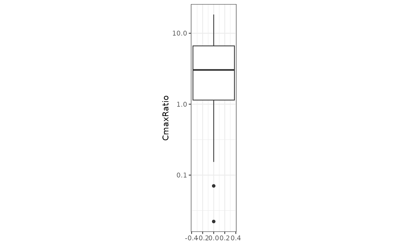
There are 21.3 % of compounds with a predicted Cmax within 2-fold of the observed value, 53.2% within 4-fold and 76.6 % within 10-fold.
We can also look at the Cmax fold ratio for the different percentiles:
tmp <- metric_results_1 %>%
  filter(Metric == "Cmax", `Metric_t1 [h]` == 0) %>%
  group_by(molecule_pref_name) %>%
  summarise(
    CmaxAvg = mean(Value, na.rm = TRUE),
    CmaxPredAvg = mean(SimMetric, na.rm = TRUE),
    CmaxRatio = mean(SimMetric / Value, na.rm = TRUE)
  ) %>%
  summarise(
    CmaxRatio5th = 2^quantile(abs(log2(CmaxRatio)), c(0.05)),
    CmaxRatio25th = 2^quantile(abs(log2(CmaxRatio)), c(0.25)),
    CmaxRatio50th = 2^quantile(abs(log2(CmaxRatio)), c(0.50)),
    CmaxRatio75th = 2^quantile(abs(log2(CmaxRatio)), c(0.75)),
    CmaxRatio95th = 2^quantile(abs(log2(CmaxRatio)), c(0.95))
  )
So we have 50% of the compound for which the AUC0Inf fold ratio is within 3.8 folds.
Comparing Cmax can be more challenging, as the sampling time points may influence the observed estimated values, and the full observed PK profiles are not available in the extracted Chembl data. It can be expected that the simulated Cmax, sampled every 10 minutes, could differ from the observed one, for which the sampling frequency and method of Cmax determination (direct observation or NCA/compartmental analysis) are not always known.
If we look more closely at the Cmax (one dot is one studies and one compound i.e. one color can have multiple studies associated), most studies/compounds are overpredicted but within 10-fold of the observed value, with one compound particularly underpredicted.
The dashed lines indicating identity (black), 2-fold (dark grey) and 10-fold (light grey) ratio.
p <- metric_results_1 %>%
  filter(Metric == "Cmax", `Metric_t1 [h]` == 0) %>%
    ggplot(aes(x = Value, y = SimMetric, color = molecule_pref_name)) +
      geom_point(show.legend = F) +
      geom_abline(slope = 1, intercept = 0) +
      labs(x = "Observed Cmax", y = "Predicted Cmax") +
      scale_x_log10() + scale_y_log10() +
      geom_abline(slope = 1, intercept = log10(2), col = "grey50", linetype = "dashed") +
      geom_abline(slope = 1, intercept = -log10(2), col = "grey50", linetype = "dashed") +
      geom_abline(slope = 1, intercept = log10(10), col = "grey80", linetype = "dashed") +
      geom_abline(slope = 1, intercept = -log10(10), col = "grey80", linetype = "dashed") +
      theme_bw()

ggplotly(p)
AUC vs Cmax
Looking at AUC and Cmax ratios together shows that in most cases, the AUC0Inf ratio and the Cmax ratio are correlated, meaning we tend to over- or underpredict both at the same time.
p <- metric_results_1 %>%
  filter((Metric == "Cmax" & `Metric_t1 [h]` == 0 ) | (Metric == "AUC" & `Metric_t1 [h]` == 0 & `Metric_t2 [h]` == Inf)) %>%
  tidyr::pivot_wider(
    id_cols = c(StudyID, ProtocolID, molecule_pref_name, canonical_smiles, Meal),
    names_from = Metric,
    values_from = c(Value, SimMetric),
    values_fn = c("Value" = ~ mean(.x), "SimMetric" = ~ mean(.x))
  ) %>%
  mutate(AUC0Inf_Ratio = SimMetric_AUC / Value_AUC,
         Cmax_Ratio = SimMetric_Cmax / Value_Cmax) %>%
  ggplot(aes(x = AUC0Inf_Ratio, y = Cmax_Ratio, color = molecule_pref_name)) +
    geom_point(show.legend = F) +
    geom_abline(slope = 1, intercept = 0) +
    labs(x = "AUC0Inf ratio", y = "Cmax ratio") +
    scale_x_log10() + scale_y_log10() +
    geom_vline(xintercept = 2, col = "grey50", linetype = "dashed") +
    geom_vline(xintercept = 0.5, col = "grey50", linetype = "dashed") +
    geom_vline(xintercept = 10, col = "grey80", linetype = "dashed") +
    geom_vline(xintercept = 0.1, col = "grey80", linetype = "dashed") +
    geom_hline(yintercept = 2, col = "grey50", linetype = "dashed") +
    geom_hline(yintercept = 0.5, col = "grey50", linetype = "dashed") +
    geom_hline(yintercept = 10, col = "grey80", linetype = "dashed") +
    geom_hline(yintercept = 0.1, col = "grey80", linetype = "dashed") +
    theme_bw()

ggplotly(p)
The dashed lines indicate the 2-fold (dark grey) and 10-fold (light grey) ratio for both AUC0Inf and Cmax.
Characteristics of compounds compared to their predictability
We can further investigate which compounds exhibit less accurate AUC and Cmax predictions to better understand the potential applicability domain of the pipeline. However, this domain is mainly constrained by the applicability of the QSAR inputs used, as well as the assumptions and limitations of the PBPK model.
Lipophilicity effect
Compounds with high or low lipophilicty values tend to be the most challenging to predict accurately. This is regularly observed in HT-PBPK assessments, as the lipophilicity is a key parameter for the distribution and absorption of compounds. The reasons can be two-fold: QSAR predictions for compounds with extreme lipophilicity may be less accurate, and PBPK models may estimate absorption and distribution less reliably in such cases.
p <- full_join(
  x = metric_results_1 %>%
    filter(Metric == "AUC" & `Metric_t1 [h]` == 0 & `Metric_t2 [h]` == Inf) %>%
    mutate(AUC0Inf_Ratio = SimMetric / Value),
  y = InputCompounds,
  by = c("molecule_pref_name", "canonical_smiles")
) %>%
  ggplot(aes(x = logD, y = AUC0Inf_Ratio, color = molecule_pref_name)) +
  geom_point() +
  geom_hline(yintercept = 2, col = "grey50", linetype = "dashed") +
  geom_hline(yintercept = 0.5, col = "grey50", linetype = "dashed") +
  geom_hline(yintercept = 10, col = "grey80", linetype = "dashed") +
  geom_hline(yintercept = 0.1, col = "grey80", linetype = "dashed") +
  scale_y_log10() +
  labs(x = "Compound logD", y = "AUC0Inf ratio") +
  theme_bw()

ggplotly(p)
We observed a trend that high lypophilic compounds have an underpredicted AUC0Inf, while low lipophilicity compounds are more overpredicted.
Fraction unbound effect
Similarly, compounds that have a very low fraction unbound are also poorly predicted. Fraction unbound tends to correlate with lipophilicity and has a significant impact on compound distribution. Even small changes in this parameter can greatly affect predicted AUC and Cmax, mainly for low fraction unbound compounds.
p <- full_join(
  x = metric_results_1 %>%
    filter(Metric == "AUC" & `Metric_t1 [h]` == 0 & `Metric_t2 [h]` == Inf) %>%
    mutate(AUC0Inf_Ratio = SimMetric / Value),
  y = InputCompounds,
  by = c("molecule_pref_name", "canonical_smiles")
) %>%
  ggplot(aes(x = Fu, y = AUC0Inf_Ratio, color = molecule_pref_name)) +
    geom_point() +
    geom_hline(yintercept = 2, col = "grey50", linetype = "dashed") +
    geom_hline(yintercept = 0.5, col = "grey50", linetype = "dashed") +
    geom_hline(yintercept = 10, col = "grey80", linetype = "dashed") +
    geom_hline(yintercept = 0.1, col = "grey80", linetype = "dashed") +
    scale_y_log10() +
    labs(x = "Compound Fraction unbound", y = "AUC0Inf ratio") +
    theme_bw()

ggplotly(p)
Solubility effect
Compounds with very low solubility are also challenging to predict accurately.
p <- full_join(
  x = metric_results_1 %>%
    filter(Metric == "AUC" & `Metric_t1 [h]` == 0 & `Metric_t2 [h]` == Inf) %>%
    mutate(AUC0Inf_Ratio = SimMetric / Value),
  y = InputCompounds,
  by = c("molecule_pref_name", "canonical_smiles")
) %>%
  ggplot(aes(x = logS, y = AUC0Inf_Ratio, color = molecule_pref_name)) +
    geom_point() +
    geom_hline(yintercept = 2, col = "grey50", linetype = "dashed") +
    geom_hline(yintercept = 0.5, col = "grey50", linetype = "dashed") +
    geom_hline(yintercept = 10, col = "grey80", linetype = "dashed") +
    geom_hline(yintercept = 0.1, col = "grey80", linetype = "dashed") +
    scale_y_log10() +
    labs(x = "Compound Solubility (logS)", y = "AUC0Inf ratio") +
    theme_bw()

ggplotly(p)
Compare with other scenarios
We can compare the results with other scenarios that use different QSAR values as input or make different assumptions (e.g., adding artificially high organ permeability or solubility).
The different scenario results are already calculated and available in the package. We will load and combine them for comparison.
for (i in 2:18) {
  path <- system.file("extdata", "Chembl_Test_Pipeline", paste0("metrics_scenario", i, ".csv"), package = "ESQhtpbpk")
  assign(x = paste0("metric_results_", i), value = read.csv(path, stringsAsFactors = FALSE, check.names = FALSE))
}

scenario_1to18 <- metric_results_1 %>% mutate(Scenario = "Scenario 1")

for (i in 2:18) {
  scenario_1to18 <- rbind(
    scenario_1to18,
    eval(parse(text = paste0("metric_results_", i))) %>%
      mutate(Scenario = paste("Scenario", i))
  )
}
Calculate and compare AUC 0 Inf ratio and Cmax of the different scenarios:
# Calculate AUC0InfRatio for all studies with it and for each scenario
tmp <- scenario_1to18 %>%
  filter(Metric == "AUC", `Metric_t1 [h]` == 0, `Metric_t2 [h]` == Inf) %>%
  group_by(molecule_pref_name, Scenario) %>%
  summarise(
    AUC0InfAvg = mean(Value, na.rm = TRUE),
    AUC0InfPredAvg = mean(SimMetric, na.rm = TRUE),
    AUC0InfRatio = mean(SimMetric / Value, na.rm = TRUE)
  )
#> `summarise()` has regrouped the output.
#> ℹ Summaries were computed grouped by molecule_pref_name and Scenario.
#> ℹ Output is grouped by molecule_pref_name.
#> ℹ Use `summarise(.groups = "drop_last")` to silence this message.
#> ℹ Use `summarise(.by = c(molecule_pref_name, Scenario))` for per-operation
#>   grouping (`?dplyr::dplyr_by`) instead.
tmp$Scenario <- factor(tmp$Scenario, levels = paste("Scenario", 1:18), ordered = TRUE)

p <- ggplot(tmp, aes(y = AUC0InfRatio, x = Scenario)) +
  geom_boxplot() +
  scale_y_log10() +
  theme_bw() +
  geom_hline(yintercept = 2, col = "grey50", linetype = "dashed") +
  geom_hline(yintercept = 0.5, col = "grey50", linetype = "dashed") +
  geom_hline(yintercept = 10, col = "grey20", linetype = "dashed") +
  geom_hline(yintercept = 0.1, col = "grey20", linetype = "dashed") +
  theme(axis.text.x = element_text(angle = 45, hjust = 1)) +
  coord_cartesian(ylim = c(0.001, 1000))
p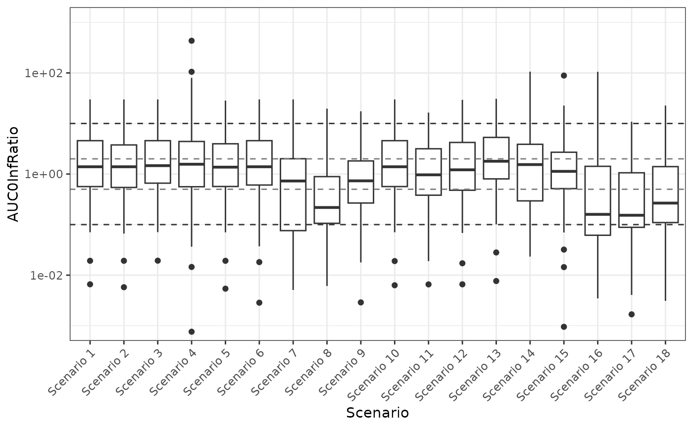
# Calculate CmaxRatio for all studies with it and for each scenario
tmp <- scenario_1to18 %>%
  filter(Metric == "Cmax", `Metric_t1 [h]` == 0) %>%
  group_by(molecule_pref_name, Scenario) %>%
  summarise(
    CmaxAvg = mean(Value, na.rm = TRUE),
    CmaxPredAvg = mean(SimMetric, na.rm = TRUE),
    CmaxRatio = mean(SimMetric / Value, na.rm = TRUE)
  )
#> `summarise()` has regrouped the output.
#> ℹ Summaries were computed grouped by molecule_pref_name and Scenario.
#> ℹ Output is grouped by molecule_pref_name.
#> ℹ Use `summarise(.groups = "drop_last")` to silence this message.
#> ℹ Use `summarise(.by = c(molecule_pref_name, Scenario))` for per-operation
#>   grouping (`?dplyr::dplyr_by`) instead.
tmp$Scenario <- factor(tmp$Scenario, levels = paste("Scenario", 1:18), ordered = TRUE)

p <- ggplot(tmp, aes(y = CmaxRatio, x = Scenario)) +
  geom_boxplot() +
  scale_y_log10() +
  theme_bw() +
  geom_hline(yintercept = 2, col = "grey50", linetype = "dashed") +
  geom_hline(yintercept = 0.5, col = "grey50", linetype = "dashed") +
  geom_hline(yintercept = 10, col = "grey20", linetype = "dashed") +
  geom_hline(yintercept = 0.1, col = "grey20", linetype = "dashed") +
  theme(axis.text.x = element_text(angle = 45, hjust = 1)) +
  coord_cartesian(ylim = c(0.001, 1000))
p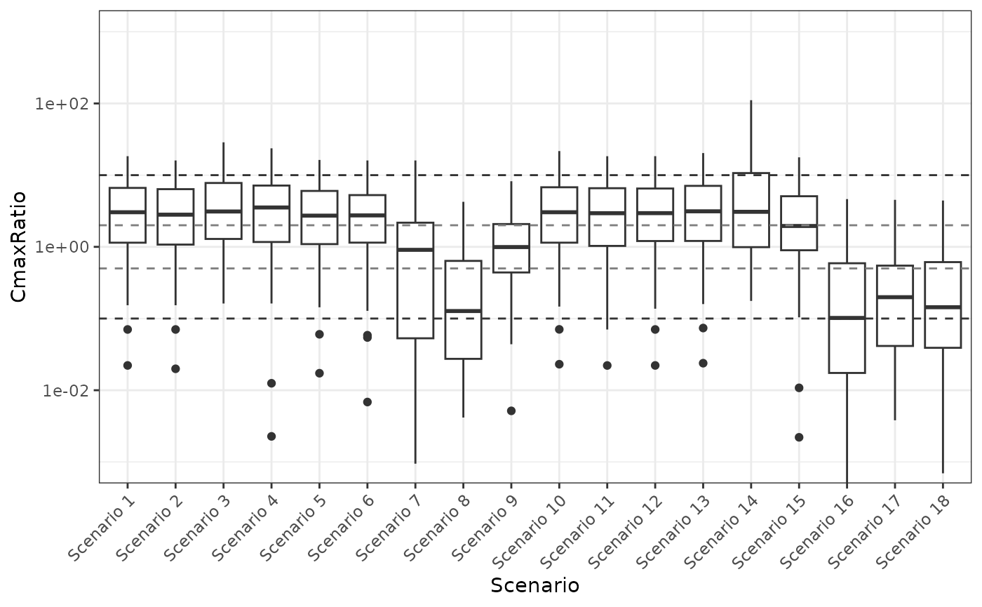
Scenario 9 (assuming high tissue permeability) and Scenario 15 (using logMA as calculated by Pearce from logP) seem to provide more reasonable AUC0Inf and Cmax predictions. Even though for Scenario 15, Cmax still tends to be overpredicted in most cases.
Let’s have a closer look at those.
Scenario 9
Scenario 9 assumes a high tissue permeability
AUC0Inf
The predicted AUC0Inf can be checked against the observed data.
The AUC0Inf for all compounds is centered slightly below 1, meaning with the high tissue permeability assumption, we tends to slightly underestimate the AUC compared to the observed value:
metric_results_9 %>%
  filter(Metric == "AUC", `Metric_t1 [h]` == 0, `Metric_t2 [h]` == Inf) %>%
  group_by(molecule_pref_name) %>%
  summarise(
    AUC0InfAvg = mean(Value, na.rm = TRUE),
    AUC0InfPredAvg = mean(SimMetric, na.rm = TRUE),
    AUC0InfRatio = mean(SimMetric / Value, na.rm = TRUE)
  ) %>%
  ggplot() +
    geom_boxplot(aes(y = AUC0InfRatio)) +
    scale_y_log10() +
    theme_bw() +
    theme(aspect.ratio = 5)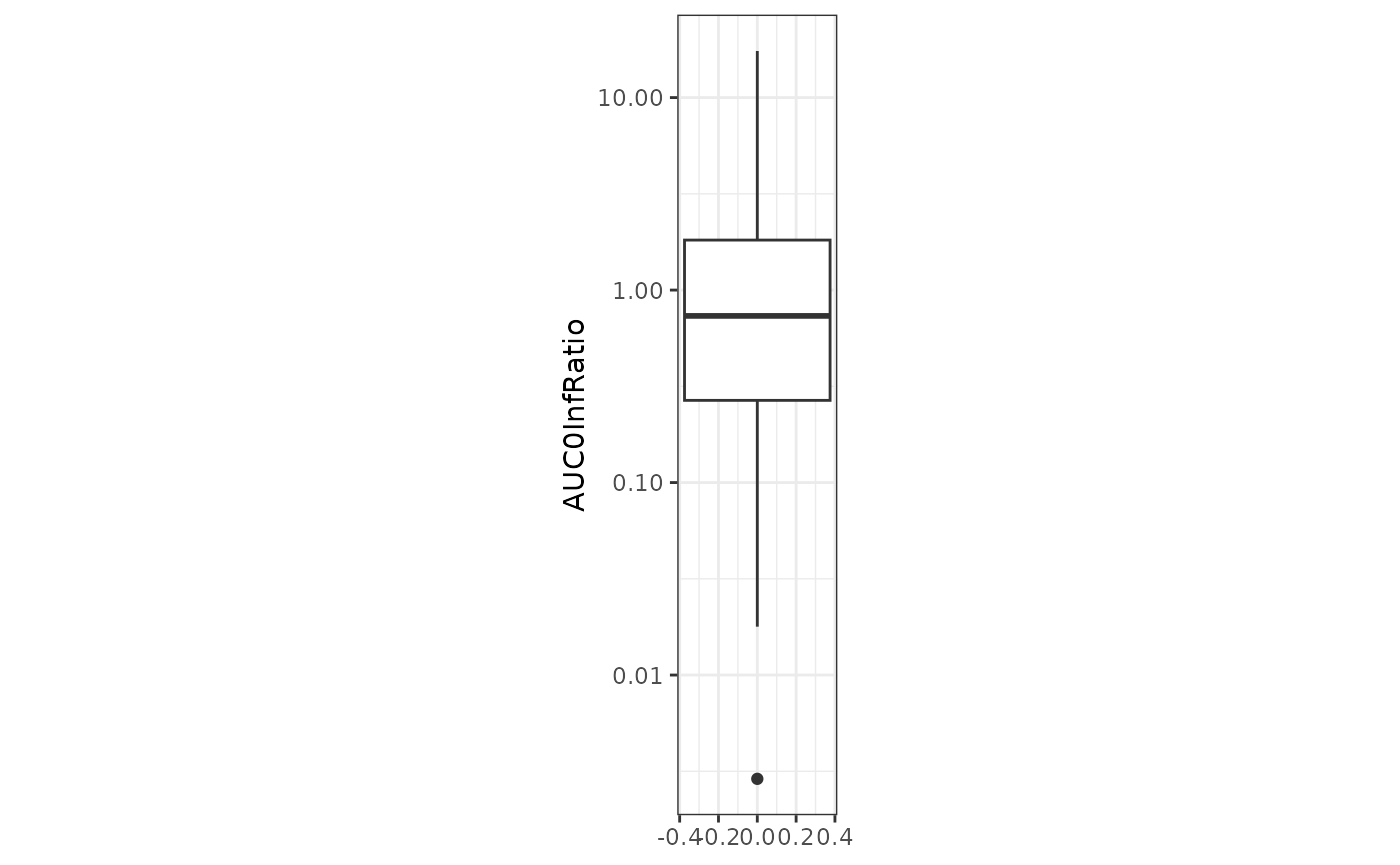
There are 42.2 % of compounds with a predicted AUC0Inf within 2-fold of the observed value, 62.2% within 4-fold and 86.7 % within 10-fold.
With this assumption it increases the number of compounds for which the AUC0Inf is within 2-fold, 4-fold and 10-fold of the observed value compared to the default scenario, at least for the tested set of compounds.
If we look more in detail at the AUC0Inf (one dot is one studies and one compound i.e. one color can have multiple studies associated), we can see that most of the studies/compounds are within 10-fold of the observed value, with one compound being particularly under-predicted.
The dashed lines indicating identity (black), 2-fold (dark grey) and 10-fold (light grey) ratio.
p <- metric_results_9 %>%
  filter(Metric == "AUC", `Metric_t1 [h]` == 0, `Metric_t2 [h]` == Inf) %>%
    ggplot(aes(x = Value, y = SimMetric, color = molecule_pref_name)) +
      geom_point(show.legend = F) +
      geom_abline(slope = 1, intercept = 0) +
      labs(x = "Observed AUC0Inf", y = "Predicted AUC0Inf") +
      scale_x_log10() + scale_y_log10() +
      geom_abline(slope = 1, intercept = log10(2), col = "grey50", linetype = "dashed") +
      geom_abline(slope = 1, intercept = -log10(2), col = "grey50", linetype = "dashed") +
      geom_abline(slope = 1, intercept = log10(10), col = "grey80", linetype = "dashed") +
      geom_abline(slope = 1, intercept = -log10(10), col = "grey80", linetype = "dashed") +
      theme_bw()

ggplotly(p)
We can see that with this assumption the AUC0Inf is much more center around the observed value.
tmp <- scenario_1to18 %>%
  filter(Metric == "AUC", `Metric_t1 [h]` == 0, `Metric_t2 [h]` == Inf) %>%
  filter(Scenario %in% c("Scenario 1", "Scenario 9")) %>%
  group_by(molecule_pref_name, Scenario, StudyID) %>%
  summarise(
    AUC0InfAvg = mean(Value, na.rm = TRUE),
    AUC0InfPredAvg = mean(SimMetric, na.rm = TRUE),
    AUC0InfRatio = mean(SimMetric / Value, na.rm = TRUE)
  ) %>%
  pivot_wider(
    id_cols = c(molecule_pref_name, StudyID),
    names_from = Scenario,
    names_prefix = "AUC0Inf Ratio - ",
    values_from = c(AUC0InfRatio)
  )
#> `summarise()` has regrouped the output.
#> ℹ Summaries were computed grouped by molecule_pref_name, Scenario, and StudyID.
#> ℹ Output is grouped by molecule_pref_name and Scenario.
#> ℹ Use `summarise(.groups = "drop_last")` to silence this message.
#> ℹ Use `summarise(.by = c(molecule_pref_name, Scenario, StudyID))` for
#>   per-operation grouping (`?dplyr::dplyr_by`) instead.

p <- ggplot(tmp, aes(x = `AUC0Inf Ratio - Scenario 1`, y = `AUC0Inf Ratio - Scenario 9`, color = molecule_pref_name)) +
  geom_point() +
  scale_x_log10() +
  scale_y_log10() +
  theme_bw() +
  geom_abline(aes(intercept = log10(2), slope = 1), col = "grey50", linetype = "dashed") +
  geom_abline(aes(intercept = -log10(2), slope = 1), col = "grey50", linetype = "dashed") +
  geom_abline(aes(intercept = log10(10), slope = 1), col = "grey20", linetype = "dashed") +
  geom_abline(aes(intercept = -log10(10), slope = 1), col = "grey20", linetype = "dashed") +
  geom_abline(aes(intercept = log10(1), slope = 1), col = "red", linetype = "dashed")

ggplotly(p)
With this assumption the AUC0Inf was decreased for a few compounds that were overpredicted, sometimes to such extent, that they became underpredicted. However, for most compounds the AUC0Inf stayed very similar to the previous scenario with less 2 fold difference between the two scenarios.
Cmax
The Cmax for all compounds is now better centered around the observed Cmax.
metric_results_9 %>%
  filter(Metric == "Cmax", `Metric_t1 [h]` == 0) %>%
  group_by(molecule_pref_name) %>%
  summarise(
    CmaxAvg = mean(Value, na.rm = TRUE),
    CmaxPredAvg = mean(SimMetric, na.rm = TRUE),
    CmaxRatio = mean(SimMetric / Value, na.rm = TRUE)
  ) %>%
  ggplot() +
    geom_boxplot(aes(y = CmaxRatio)) +
    scale_y_log10() +
    theme_bw() +
    theme(aspect.ratio = 5)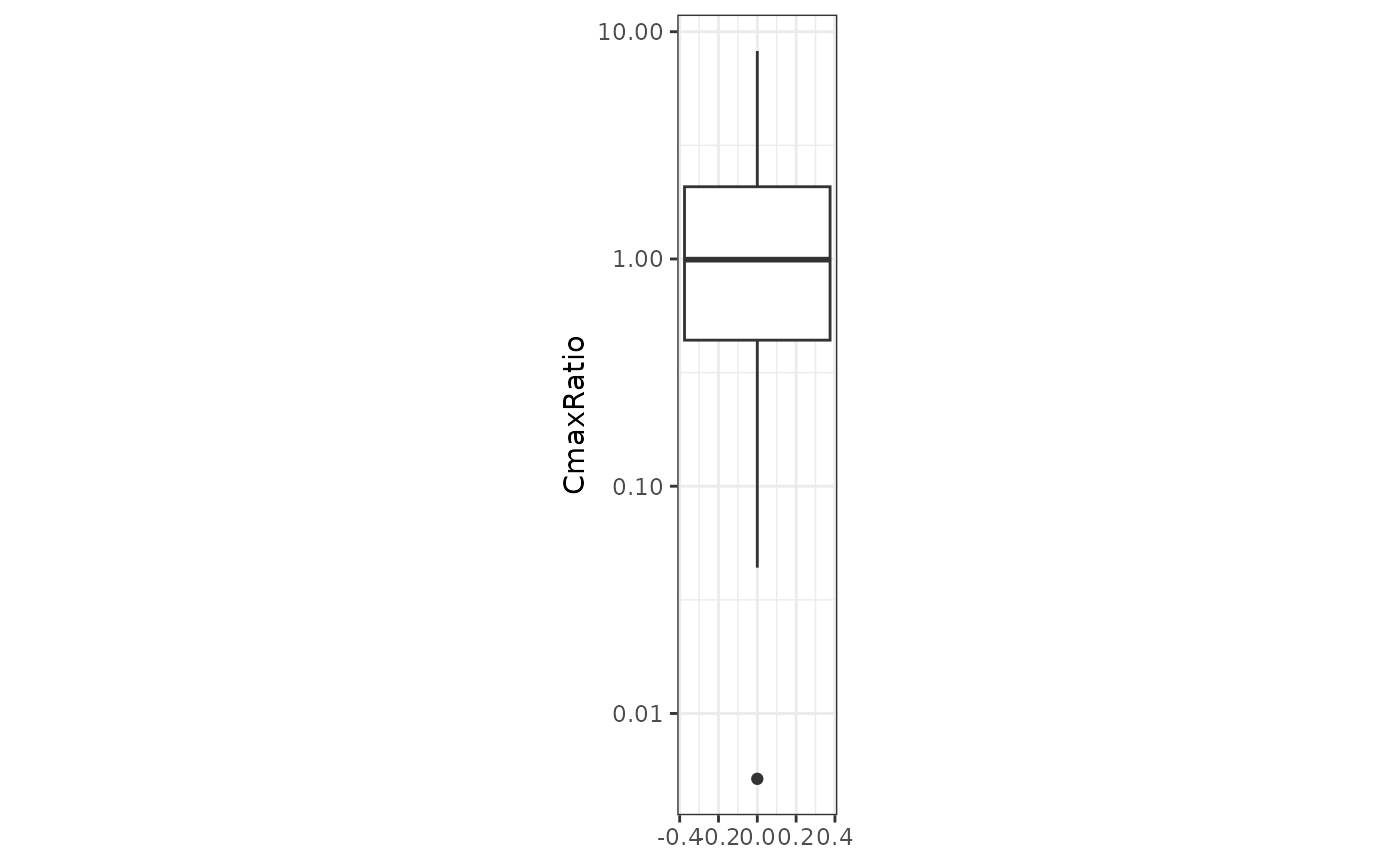
There are 42.6 % of compounds with a predicted Cmax within 2-fold of the observed value, 72.3% within 4-fold and 93.6 % within 10-fold.
With this assumption, the number of compounds for which Cmax is within 2-fold, 4-fold, and 10-fold of the observed value increases compared to the default scenario.
The dashed lines indicating identity (black), 2-fold (dark grey) and 10-fold (light grey) ratio.
p <- metric_results_9 %>%
  filter(Metric == "Cmax", `Metric_t1 [h]` == 0) %>%
    ggplot(aes(x = Value, y = SimMetric, color = molecule_pref_name)) +
      geom_point(show.legend = F) +
      geom_abline(slope = 1, intercept = 0) +
      labs(x = "Observed Cmax", y = "Predicted Cmax") +
      scale_x_log10() + scale_y_log10() +
      geom_abline(slope = 1, intercept = log10(2), col = "grey50", linetype = "dashed") +
      geom_abline(slope = 1, intercept = -log10(2), col = "grey50", linetype = "dashed") +
      geom_abline(slope = 1, intercept = log10(10), col = "grey80", linetype = "dashed") +
      geom_abline(slope = 1, intercept = -log10(10), col = "grey80", linetype = "dashed") +
      theme_bw()

ggplotly(p)
We can see that with this assumption the Cmax is much more center around the observed value.
tmp <- scenario_1to18 %>%
  filter(Metric == "Cmax", `Metric_t1 [h]` == 0) %>%
  filter(Scenario %in% c("Scenario 1", "Scenario 9")) %>%
  group_by(molecule_pref_name, Scenario, StudyID) %>%
  summarise(
    CmaxAvg = mean(Value, na.rm = TRUE),
    CmaxPredAvg = mean(SimMetric, na.rm = TRUE),
    CmaxRatio = mean(SimMetric / Value, na.rm = TRUE)
  ) %>%
  pivot_wider(
    id_cols = c(molecule_pref_name, StudyID),
    names_from = Scenario,
    names_prefix = "Cmax Ratio - ",
    values_from = c(CmaxRatio)
  )
#> `summarise()` has regrouped the output.
#> ℹ Summaries were computed grouped by molecule_pref_name, Scenario, and StudyID.
#> ℹ Output is grouped by molecule_pref_name and Scenario.
#> ℹ Use `summarise(.groups = "drop_last")` to silence this message.
#> ℹ Use `summarise(.by = c(molecule_pref_name, Scenario, StudyID))` for
#>   per-operation grouping (`?dplyr::dplyr_by`) instead.

p <- ggplot(tmp, aes(x = `Cmax Ratio - Scenario 1`, y = `Cmax Ratio - Scenario 9`, color = molecule_pref_name)) +
  geom_point() +
  scale_x_log10() +
  scale_y_log10() +
  theme_bw() +
  geom_abline(aes(slope = 1, intercept = log10(2)), col = "grey50", linetype = "dashed") +
  geom_abline(aes(slope = 1, intercept = -log10(2)), col = "grey50", linetype = "dashed") +
  geom_abline(aes(slope = 1, intercept = log10(10)) , col = "grey20", linetype = "dashed") +
  geom_abline(aes(slope = 1, intercept = -log10(10)) , col = "grey20", linetype = "dashed") +
  geom_abline(aes(slope = 1, intercept = log10(1)) , col = "red", linetype = "dashed")

ggplotly(p)
With this assumption the Cmax was decreased for most compounds, overall bringing most compounds closer to the observed value and mostly within 10-fold.
full_join(
  x = tmp %>%
    group_by(molecule_pref_name) %>%
    summarise(Scen9vs1Change = mean(`Cmax Ratio - Scenario 9` / `Cmax Ratio - Scenario 1`, na.rm = T)) ,
  y = InputCompounds,
  by = c("molecule_pref_name")
) %>%
  ggplot(aes(y = `Scen9vs1Change`, x = `MW`)) +
  geom_point() +
  geom_hline(yintercept = 2, col = "grey50", linetype = "dashed") +
  geom_hline(yintercept = 0.5, col = "grey50", linetype = "dashed") +
  geom_hline(yintercept = 10, col = "grey80", linetype = "dashed") +
  geom_hline(yintercept = 0.1, col = "grey80", linetype = "dashed") +
  scale_y_log10() +
  labs(x = "Molecular weight", y = "Scenario 9 vs Scenario 1 - Cmax change") +
  theme_bw()
#> Warning: Removed 1 row containing missing values or values outside the scale range
#> (`geom_point()`).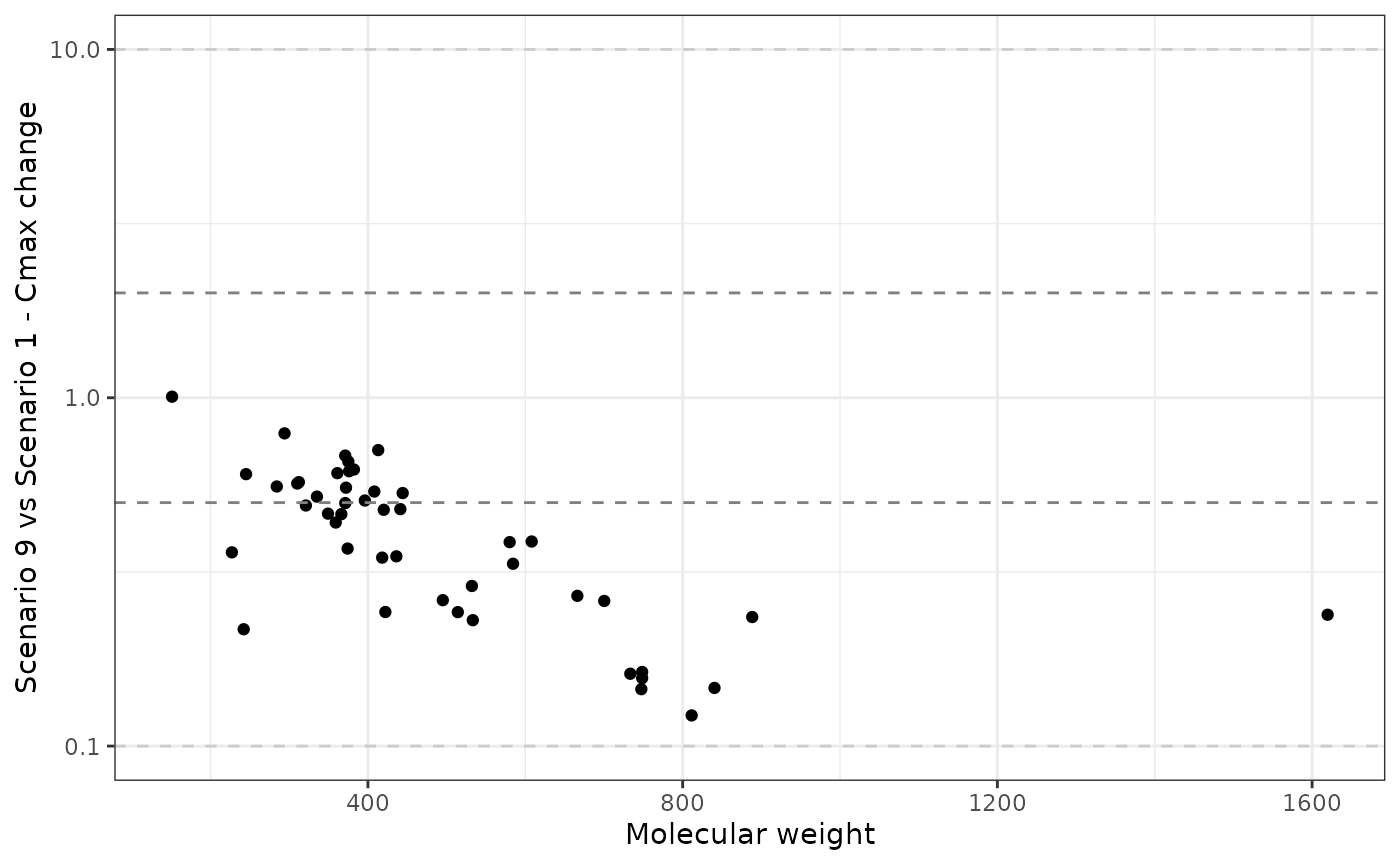
The Cmax is more strongly reduced for compounds with a higher molecular weight.
Scenario 15
Scenario 15 uses transforms logP to LogMA as calculated by Pearce
AUC0Inf
The predicted AUC0Inf can be check with observed data.
The AUC0Inf for all compounds is centered around 1, meaning with this input for lipophilicity the simulated AUC0Inf around the observed value:
metric_results_15 %>%
  filter(Metric == "AUC", `Metric_t1 [h]` == 0, `Metric_t2 [h]` == Inf) %>%
  group_by(molecule_pref_name) %>%
  summarise(
    AUC0InfAvg = mean(Value, na.rm = TRUE),
    AUC0InfPredAvg = mean(SimMetric, na.rm = TRUE),
    AUC0InfRatio = mean(SimMetric / Value, na.rm = TRUE)
  ) %>%
  ggplot() +
    geom_boxplot(aes(y = AUC0InfRatio)) +
    scale_y_log10() +
    theme_bw() +
    theme(aspect.ratio = 5)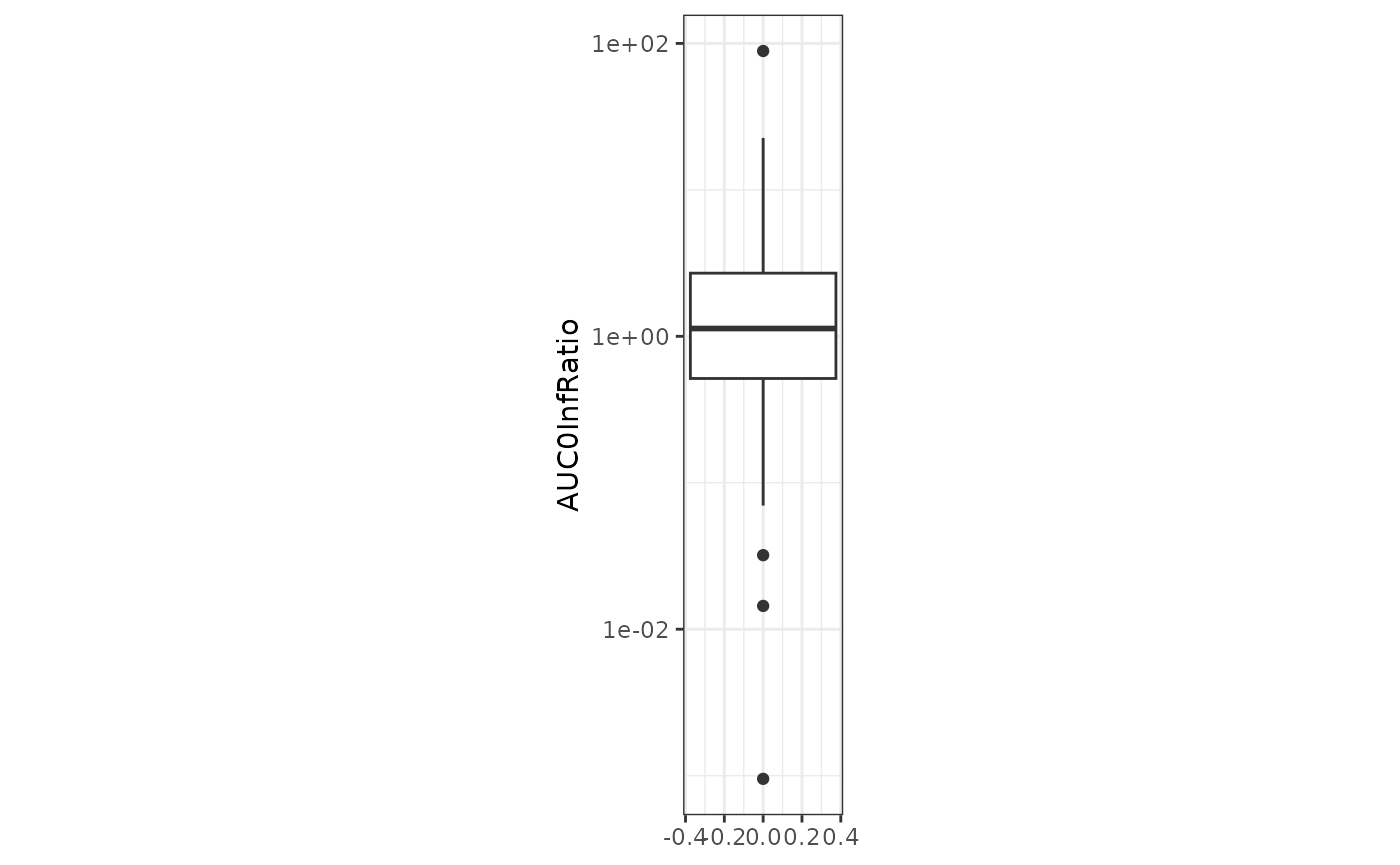
There are 35.6 % of compounds with a predicted AUC0Inf within 2-fold of the observed value, 62.2% within 4-fold and 75.6 % within 10-fold.
With this assumption it increase (but only very slightly) the number of compounds for which the AUC0Inf is within 2-fold, 4-fold and 10-fold of the observed value compared to the default scenario, at least for the tested set of compounds.
If we look more in detail at the AUC0Inf (one dot is one studies and one compound i.e. one color can have multiple studies associated), we can see that most of the studies/compounds are within 10-fold of the observed value, with one compound being particularly underpredicted.
The dashed lines indicating identity (black), 2-fold (dark grey) and 10-fold (light grey) ratio.
p <- metric_results_15 %>%
  filter(Metric == "AUC", `Metric_t1 [h]` == 0, `Metric_t2 [h]` == Inf) %>%
    ggplot(aes(x = Value, y = SimMetric, color = molecule_pref_name)) +
      geom_point(show.legend = F) +
      geom_abline(slope = 1, intercept = 0) +
      labs(x = "Observed AUC0Inf", y = "Predicted AUC0Inf") +
      scale_x_log10() + scale_y_log10() +
      geom_abline(slope = 1, intercept = log10(2), col = "grey50", linetype = "dashed") +
      geom_abline(slope = 1, intercept = -log10(2), col = "grey50", linetype = "dashed") +
      geom_abline(slope = 1, intercept = log10(10), col = "grey80", linetype = "dashed") +
      geom_abline(slope = 1, intercept = -log10(10), col = "grey80", linetype = "dashed") +
      theme_bw()

ggplotly(p)
tmp <- scenario_1to18 %>%
  filter(Metric == "AUC", `Metric_t1 [h]` == 0, `Metric_t2 [h]` == Inf) %>%
  filter(Scenario %in% c("Scenario 1", "Scenario 15")) %>%
  group_by(molecule_pref_name, Scenario, StudyID) %>%
  summarise(
    AUC0InfAvg = mean(Value, na.rm = TRUE),
    AUC0InfPredAvg = mean(SimMetric, na.rm = TRUE),
    AUC0InfRatio = mean(SimMetric / Value, na.rm = TRUE)
  ) %>%
  pivot_wider(
    id_cols = c(molecule_pref_name, StudyID),
    names_from = Scenario,
    names_prefix = "AUC0Inf Ratio - ",
    values_from = c(AUC0InfRatio)
  )
#> `summarise()` has regrouped the output.
#> ℹ Summaries were computed grouped by molecule_pref_name, Scenario, and StudyID.
#> ℹ Output is grouped by molecule_pref_name and Scenario.
#> ℹ Use `summarise(.groups = "drop_last")` to silence this message.
#> ℹ Use `summarise(.by = c(molecule_pref_name, Scenario, StudyID))` for
#>   per-operation grouping (`?dplyr::dplyr_by`) instead.

p <- ggplot(tmp, aes(x = `AUC0Inf Ratio - Scenario 1`, y = `AUC0Inf Ratio - Scenario 15`, color = molecule_pref_name)) +
  geom_point() +
  scale_x_log10() +
  scale_y_log10() +
  theme_bw() +
  geom_abline(aes(intercept = log10(2), slope = 1), col = "grey50", linetype = "dashed") +
  geom_abline(aes(intercept = -log10(2), slope = 1), col = "grey50", linetype = "dashed") +
  geom_abline(aes(intercept = log10(10), slope = 1), col = "grey20", linetype = "dashed") +
  geom_abline(aes(intercept = -log10(10), slope = 1), col = "grey20", linetype = "dashed") +
  geom_abline(aes(intercept = -log10(1), slope = 1), col = "red", linetype = "dashed")
ggplotly(p)
The AUC0Inf is only modified for some compounds, sometimes slightly increase sometimes slightly decrease compared to the default scenario.
Cmax
Similarly we can also look at other metrics such as Cmax. The Cmax for all compounds is well center around the observed Cmax this this assumption.
metric_results_15 %>%
  filter(Metric == "Cmax", `Metric_t1 [h]` == 0) %>%
  group_by(molecule_pref_name) %>%
  summarise(
    CmaxAvg = mean(Value, na.rm = TRUE),
    CmaxPredAvg = mean(SimMetric, na.rm = TRUE),
    CmaxRatio = mean(SimMetric / Value, na.rm = TRUE)
  ) %>%
  ggplot() +
    geom_boxplot(aes(y = CmaxRatio)) +
    scale_y_log10() +
    theme_bw() +
    theme(aspect.ratio = 5) + coord_cartesian(ylim = c(0.001, 50))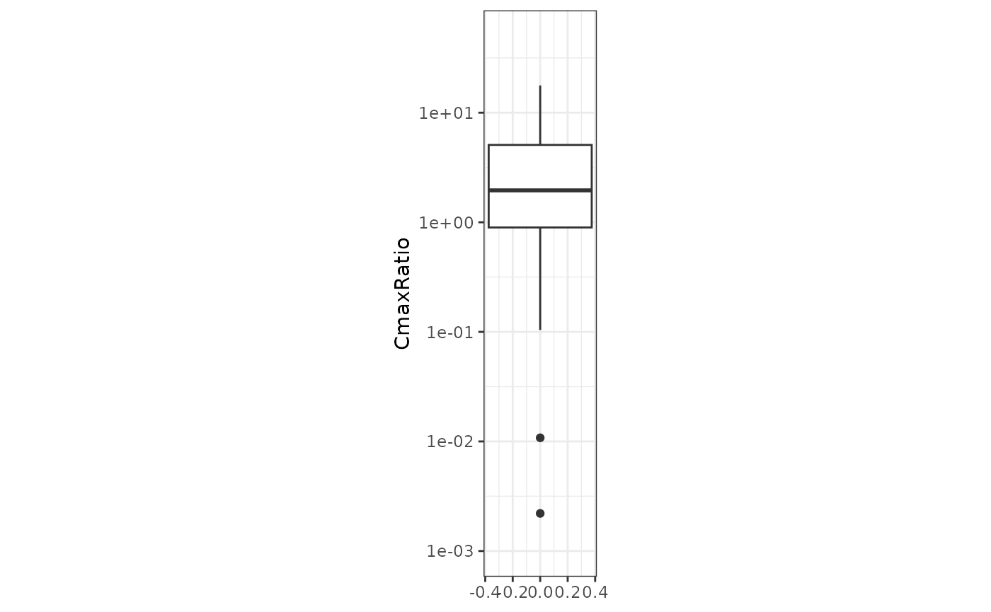
There are 29.8 % of compounds with a predicted Cmax within 2-fold of the observed value, 51.1% within 4-fold and 80.9 % within 10-fold.
With this assumption it slightly increase the number of compounds for which the Cmax is within 2-fold and 10-fold but not 4-fold of the observed value compared to the default scenario, at least for the tested set of compounds.
If we look more in detail at the Cmax (one dot is one studies and one compound i.e. one color can have multiple studies associated), we can see that most of the studies/compounds are overpredicted but within 10-fold of the observed value, with one compound being particularly underpredicted.
The dashed lines indicating identity (black), 2-fold (dark grey) and 10-fold (light grey) ratio.
p <- metric_results_15 %>%
  filter(Metric == "Cmax", `Metric_t1 [h]` == 0) %>%
    ggplot(aes(x = Value, y = SimMetric, color = molecule_pref_name)) +
      geom_point(show.legend = F) +
      geom_abline(slope = 1, intercept = 0) +
      labs(x = "Observed Cmax", y = "Predicted Cmax") +
      scale_x_log10() + scale_y_log10() +
      geom_abline(slope = 1, intercept = log10(2), col = "grey50", linetype = "dashed") +
      geom_abline(slope = 1, intercept = -log10(2), col = "grey50", linetype = "dashed") +
      geom_abline(slope = 1, intercept = log10(10), col = "grey80", linetype = "dashed") +
      geom_abline(slope = 1, intercept = -log10(10), col = "grey80", linetype = "dashed") +
      theme_bw()

ggplotly(p)
The improvement on Cmax with this assumption is not particularly striking.
tmp <- scenario_1to18 %>%
  filter(Metric == "Cmax", `Metric_t1 [h]` == 0) %>%
  filter(Scenario %in% c("Scenario 1", "Scenario 15")) %>%
  group_by(molecule_pref_name, Scenario, StudyID) %>%
  summarise(
    CmaxAvg = mean(Value, na.rm = TRUE),
    CmaxPredAvg = mean(SimMetric, na.rm = TRUE),
    CmaxRatio = mean(SimMetric / Value, na.rm = TRUE)
  ) %>%
  pivot_wider(
    id_cols = c(molecule_pref_name, StudyID),
    names_from = Scenario,
    names_prefix = "Cmax Ratio - ",
    values_from = c(CmaxRatio)
  )
#> `summarise()` has regrouped the output.
#> ℹ Summaries were computed grouped by molecule_pref_name, Scenario, and StudyID.
#> ℹ Output is grouped by molecule_pref_name and Scenario.
#> ℹ Use `summarise(.groups = "drop_last")` to silence this message.
#> ℹ Use `summarise(.by = c(molecule_pref_name, Scenario, StudyID))` for
#>   per-operation grouping (`?dplyr::dplyr_by`) instead.

p <- ggplot(tmp, aes(x = `Cmax Ratio - Scenario 1`, y = `Cmax Ratio - Scenario 15`, color = molecule_pref_name)) +
  geom_point() +
  scale_x_log10() +
  scale_y_log10() +
  theme_bw() +
  geom_abline(aes(slope = 1, intercept = log10(2)), col = "grey50", linetype = "dashed") +
  geom_abline(aes(slope = 1, intercept = -log10(2)), col = "grey50", linetype = "dashed") +
  geom_abline(aes(slope = 1, intercept = log10(10)), col = "grey20", linetype = "dashed") +
  geom_abline(aes(slope = 1, intercept = -log10(10)), col = "grey20", linetype = "dashed") +
  geom_abline(aes(slope = 1, intercept = log10(1)), col = "red", linetype = "dashed")
ggplotly(p)
The Cmax with this assumption is modified only slighly with most cmpounds exhibiting a change of less than 2 folds, except for a few of them that are significantly decreased even though they were already underpredicted.
full_join(
  x = tmp %>%
    group_by(molecule_pref_name) %>%
    summarise(Scen15vs1Change = mean(`Cmax Ratio - Scenario 15` / `Cmax Ratio - Scenario 1`, na.rm = T)) ,
  y = InputCompounds,
  by = c("molecule_pref_name")
) %>%
  ggplot(aes(x = `logD`, y = Scen15vs1Change)) +
  geom_point() +
  geom_hline(yintercept = 2, col = "grey50", linetype = "dashed") +
  geom_hline(yintercept = 0.5, col = "grey50", linetype = "dashed") +
  geom_hline(yintercept = 10, col = "grey80", linetype = "dashed") +
  geom_hline(yintercept = 0.1, col = "grey80", linetype = "dashed") +
  scale_y_log10() +
  labs(x = "Compound logD", y = "Scenario 15 vs Scenario 1 - Cmax Change") +
  theme_bw()
#> Warning: Removed 1 row containing missing values or values outside the scale range
#> (`geom_point()`).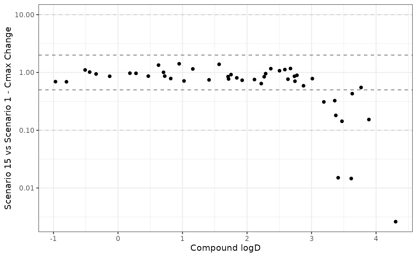
We can see that high logD compounds are more strongly affected by this change, with a decrease of Cmax, even though those were already under-predicted. So this assumption only benefits few compounds while being detrimental for high lipophilicity compound that were already poorly predicted.
Conclusion
The ESQhtpbpk package allows easy simulation of compound pharmacokinetics. The prediction results depend on the accuracy of the input data (e.g., QSAR values used) as well as the PBPK model and its assumptions. Predictions tend to be less reliable for compounds with extreme lipophilicity, low fraction unbound, and low solubility. However, given the variability of the aggregated metrics AUC0Inf and Cmax, as well as differences in sampling time points, comparisons with predicted values may not always be appropriate. Availability of full observed PK profiles would allow better harmonization of these metrics between observed and simulated data.